A/B Testing LLM Prompts: The Statistical Playbook (2026)
A/B testing LLM prompts without power analysis is theater. The 2026 playbook: MDE, sample sizing, matched pairs, bootstrap CIs, bandits, and rollout.
Table of Contents
A team rolls out a 12-line tweak to the support agent’s groundedness prompt. The offline suite of 30 examples comes back +0.02 on Groundedness. Someone calls it a win. The change ships. Twelve hours later refusal rate on legitimate refund queries is up 14 points and on-call is rolling back from a Slack thread.
That +0.02 was noise wearing a confidence interval. The dataset was too small to detect anything smaller than +0.08. Nobody computed the minimum detectable effect. Nobody ran a paired test. Nobody bootstrapped a CI on the delta. The decision was a vibe with a mean attached.
A/B testing prompts without sample-size math is theater. The right test is power analysis plus matched-pair eval plus a bootstrap CI on the delta. Most teams ship a “winning” prompt that had a 0.02 better score on 30 examples and call it shipped. This guide is the statistical playbook for the test that survives a post-mortem: MDE, sample sizing, the matched-pair design, bootstrap CIs, bandits when N=300 is too slow, and the shadow-canary-ramp sequence that gets the change to production without the 3pm rollback.
TL;DR: the test that survives a post-mortem
| Step | Decision | Rule |
|---|---|---|
| 1. Pick the MDE | What size delta matters? | Set it before you look at data. Below 0.02 is rarely worth shipping. |
| 2. Sample size from power | n_per_arm = 16 * sigma_squared / MDE_squared | Continuous rubric. Substitute p(1-p) for binary. |
| 3. Matched pairs, not groups | Same inputs, both prompts | One to two orders of magnitude tighter CI. |
| 4. Pairwise judging | Judge sees A and B together | Removes absolute-scale drift; reduces noise floor. |
| 5. Bootstrap CI on the delta | 10,000 resamples of paired deltas | Ship only when the CI sits entirely on one side of zero. |
| 6. Bandit if you have to | Thompson Sampling on >=3 arms | When regret is bounded and you cannot wait for fixed N. |
| 7. Shadow -> canary -> ramp | 0% -> 1-5% -> 25% -> 100% | Eval-gated rollback at every stage. |
Skim everything below for the math. The hard part of A/B testing prompts is not the test. It’s deciding when the result is real.
Where the theater starts: 30 examples, no power
The default failure mode is small N. A team writes 30 prompts they think cover the domain, runs both variants, reports a +0.03 mean delta on Groundedness, and ships. The sample math says that test could not have resolved anything smaller than a +0.10 delta on a typical Groundedness rubric. The +0.03 sits inside the noise band. You will fail to replicate it half the time you rerun the exact same dataset.
The fix is upstream of the test. Compute the minimum detectable effect (MDE) before you run anything. MDE is the smallest delta your test can reliably distinguish from zero at the sample size you have. Pretending the MDE doesn’t exist is what produces the 0.02 win that didn’t survive contact with production.
For a continuous rubric (a 0-1 Groundedness score, a 1-5 helpfulness score):
n_per_arm = 16 * sigma_squared / MDE_squared # alpha 0.05, power 0.80For a binary pass/fail rubric (citation valid, refusal correct):
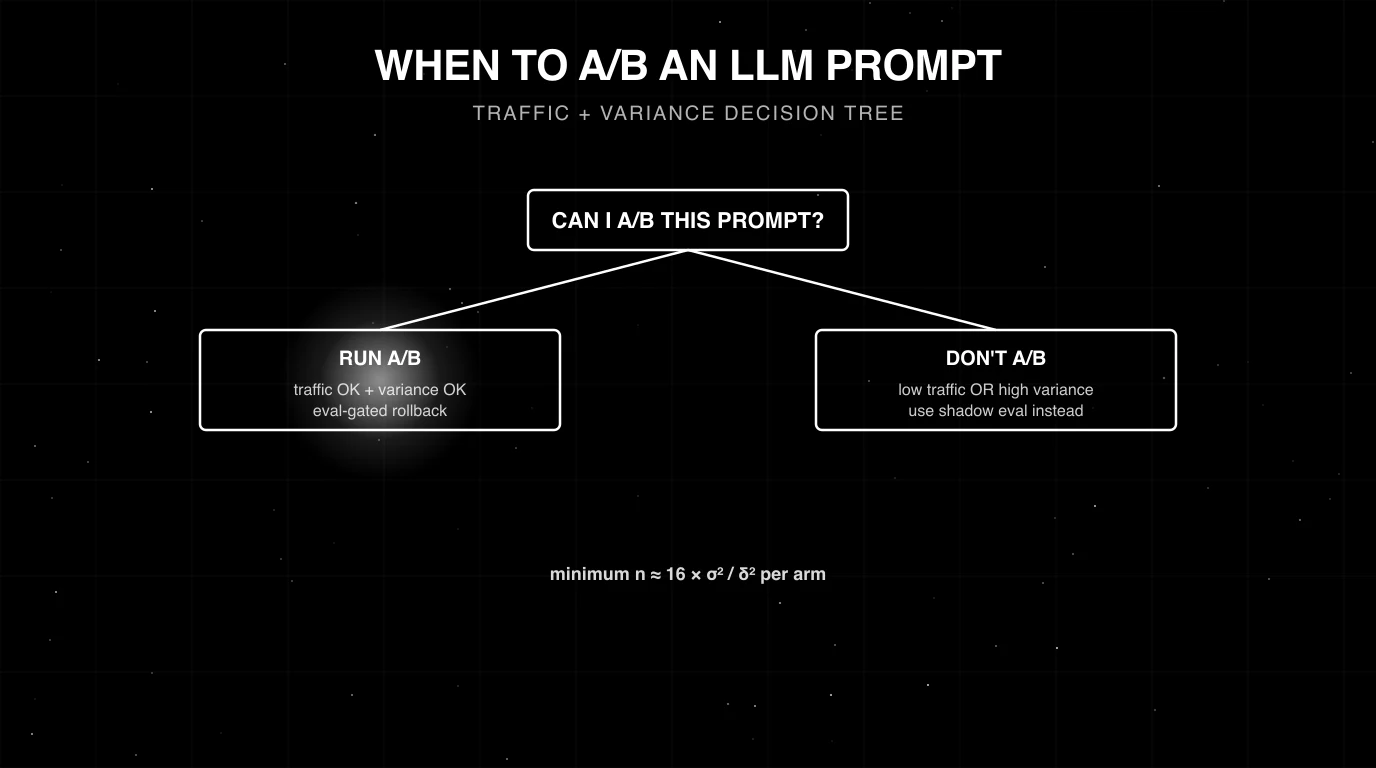
n_per_arm = 16 * p * (1 - p) / MDE_squaredThe factor of 16 is the two-sided Z-test combination at 80 percent power and 5 percent alpha. The two inputs that matter are sigma (or p) and MDE. Both have to come from somewhere.
sigma comes from a small calibration run on the rubric you’re using. Score 50-100 examples once, take the standard deviation of the per-example scores, that’s your sigma. Most calibrated LLM judges land somewhere between 0.12 and 0.25 on a 0-1 rubric.
MDE is the call you have to make: what size improvement actually matters? A 0.04 lift on Groundedness is roughly the difference between “fine” and “ship”. A 0.01 lift is below the noise floor of human review. Pick the MDE you would defend to the head of eng.
Worked numbers. Sigma 0.18, MDE 0.04: 16 * 0.0324 / 0.0016 = 324 paired examples per arm. Drop the MDE to 0.02 and the requirement jumps to 1,296 per arm. Half the MDE, four times the data; that’s the geometry of statistical resolution. Anything below 100 paired examples is below the resolution of a credible LLM A/B regardless of the model you’re testing.
The matched-pair design (this is where the test wins)
Independent groups (A gets examples 1-100, B gets 101-200) waste statistical power. The variance dominating the delta is between-example variance. Some inputs are just harder; you cannot tell whether B is better or whether B got the easier draw.
Matched-pair design runs both prompts on the same inputs and analyzes the per-example delta vector. The between-example variance cancels. What’s left is the variance of the difference, which is much smaller, sometimes one to two orders of magnitude smaller for LLM rubrics.
# Matched pairs: same inputs, both prompts, paired delta
import numpy as np
from scipy import stats

def matched_pair_test(scores_a: list[float], scores_b: list[float]):
    """Paired two-sided test on per-example deltas (B - A)."""
    assert len(scores_a) == len(scores_b), "matched pairs only"
    deltas = np.array(scores_b) - np.array(scores_a)
    mean_delta = deltas.mean()
    # Paired t-test (use Wilcoxon signed-rank if deltas are non-normal)
    t_stat, p = stats.ttest_rel(scores_b, scores_a)
    return {
        "mean_delta": float(mean_delta),
        "p_value": float(p),
        "n_pairs": len(deltas),
        "deltas": deltas,
    }
The practical consequence: a matched-pair test on 300 examples gives you the resolution an independent test would need 1,200 examples to match. Inference cost roughly doubles (you score every example twice), which is almost always cheaper than four times the examples plus four times the judge bill.
This is the single biggest win in this guide. If you change one thing, change to matched pairs.
Pointwise vs pairwise judging (and when to use each)
Two ways to score a matched pair.
Pointwise: score each output independently against a rubric (Groundedness, Completeness). Take the per-example delta. Use this when the rubric is operationally meaningful on its own (your CI gate compares against a Groundedness floor; you want the same number) and when the rubric maps to a concrete failure mode the change targets.
Pairwise (arena judging): the judge sees output A and output B for the same input and picks a winner. The score is a win rate, not a number. Use this when absolute-scale drift is the dominant noise source, when the rubric is subjective (helpfulness, tone), or when you specifically want to know which prompt is “better” rather than which scores higher on a specific dimension.
Pairwise wins on noise for most subjective rubrics: the judge anchors on the comparison, which removes a chunk of the grader’s drift between runs. Pointwise wins when you need the score itself for downstream gating. For an A/B that decides ship or not, pairwise is usually the right tool; for an A/B that needs to clear a specific floor (Groundedness >= 0.85), pointwise stays.
A clean rule: if your decision is “is B better than A”, use pairwise. If your decision is “does B clear the bar”, use pointwise. The LLM Arena as a Judge post covers the pairwise machinery in depth.
Bootstrap CIs on the delta (not the aggregate)
Mean delta plus a p-value is the second-most common A/B mistake. The p-value tells you the delta is unlikely under the null. It tells you nothing about how big the delta might actually be, which is what determines whether to ship.
Bootstrap the confidence interval on the paired-delta vector. Ten thousand resamples; take the 2.5th and 97.5th percentiles. If the 95 percent CI sits entirely on one side of zero, you have a directional win; the lower bound tells you the smallest credible improvement.
import numpy as np

def bootstrap_delta_ci(deltas: np.ndarray, n_boot: int = 10_000, alpha: float = 0.05):
    """Percentile bootstrap CI on the mean of paired deltas."""
    rng = np.random.default_rng(42)
    n = len(deltas)
    boot_means = np.empty(n_boot)
    for i in range(n_boot):
        sample = rng.choice(deltas, size=n, replace=True)
        boot_means[i] = sample.mean()
    lo, hi = np.percentile(boot_means, [100 * alpha / 2, 100 * (1 - alpha / 2)])
    return {
        "mean_delta": float(deltas.mean()),
        "ci_lo": float(lo),
        "ci_hi": float(hi),
        "ship": lo > 0,   # entirely positive CI
    }
Three rules of thumb on the CI.
If the CI straddles zero, the prompt is not better than the incumbent at 95 percent confidence regardless of how positive the mean looks. Iterate or stop.
If the CI is entirely positive but the lower bound is below your MDE, the test is underpowered for the decision you wanted to make. Add data or accept a smaller MDE.
If the CI is entirely positive and the lower bound clears your MDE, ship the change to canary. The matched-pair design plus bootstrap CI is the test result you would defend in a post-mortem.
Bootstrap is the right tool because LLM eval distributions are rarely normal. Groundedness distributions are heavily skewed toward the high end; Completeness is bimodal on routes with mixed coverage. The parametric assumptions of a plain t-test break on these shapes. Bootstrap respects whatever the data actually looks like.
Bandits, when you cannot wait for N=300
Fixed A/B works when you have two arms, time, and patience. Bandits earn their keep when neither of the last two holds.
Multi-arm bandits allocate traffic dynamically: arms that look better get more traffic; arms that look worse get less. The trade is regret (opportunity cost of serving the losing arm) against information (you still need samples to learn). Thompson Sampling is the default; it samples each arm from a posterior over its quality and serves the arm with the highest sampled value.
For binary metrics, model each arm as Beta-Bernoulli. For continuous rubrics, model each arm as Normal with conjugate updates on the mean.
import numpy as np

class BetaThompsonBandit:
    """Thompson Sampling for binary pass/fail rubrics. n_arms >= 2."""
    def __init__(self, n_arms: int, prior_alpha: float = 1.0, prior_beta: float = 1.0):
        self.alpha = np.full(n_arms, prior_alpha)
        self.beta = np.full(n_arms, prior_beta)

    def select_arm(self, rng: np.random.Generator) -> int:
        samples = rng.beta(self.alpha, self.beta)
        return int(np.argmax(samples))

    def update(self, arm: int, reward: int) -> None:
        self.alpha[arm] += reward          # 1 if rubric passed
        self.beta[arm] += (1 - reward)     # 1 if rubric failed
Use a bandit when:
- You have three or more prompt variants and want the winner converged on automatically.
- Regret is bounded (a “worse” arm is still serving usable output, not breaking).
- The cost of waiting for a fixed-N test outweighs the cost of less clean effect-size estimates.
Don’t use a bandit when you need a defensible point estimate of “B beats A by X percent”, when arms perform similarly (convergence is slow), or when you want a post-mortem-ready number to take to leadership. For two-arm decisions with time to run, fixed A/B with matched pairs and bootstrap CI is cleaner.
The systematic alternative: optimize, don’t A/B
Most teams treat A/B testing as the way to improve a prompt: write a new variant, test it, ship if it wins. The implicit assumption is that the engineer’s intuition produces good variants. Sometimes it does. Often the search space is bigger than intuition explores.
If you have an evaluator you trust and a labeled dataset, a prompt optimizer will outwork most teams’ manual A/B loops. The optimizer searches the prompt space against your scoring function instead of testing one human-authored variant at a time. agent-opt ships six optimizers covering the major paradigms: ProTeGi (gradient-style critique, learns from failures), GEPA (genetic, evolves a population), MetaPrompt (self-reflective), BayesianSearch (Bayesian over a prompt template space), RandomSearch (the honest baseline), PromptWizard (hybrid).
The pattern: keep A/B for the final ship decision (the optimizer’s winner versus the production incumbent, matched pairs plus bootstrap CI). Use the optimizer to generate the candidate instead of writing it by hand. The combination is faster than manual iteration and produces variants you would not have written.
The production rollout: shadow, canary, ramp
The offline A/B told you B beats A on a held-out dataset. Production tells you whether the dataset still represents production. The rollout sequence is shadow first, canary second, ramp third.
Shadow. Run the new prompt against live inputs without serving its output. The current prompt serves users; a shadow worker scores both prompts on the same input. Compare to the offline A/B prediction. If the production shadow delta is inside the offline CI, the dataset was representative and you can promote to canary. If it’s outside, the offline dataset missed something; pull the production traffic from the shadow window into the eval set and rerun the offline A/B before promoting.
Canary. Serve the new prompt to 1-5 percent of cohort traffic. Cohort-stable hashing (hash user-id or tenant-id modulo bucket count) so a user stays in the same arm across requests. Wire eval-gated rollback: a 15-minute rolling per-rubric pass rate, auto-revert if any monitored rubric drops below 1.5 times the rubric’s noise floor relative to the incumbent. The canary catches the regressions the offline test couldn’t see (latency, refusal distribution, edge-case routing).
Ramp. Grow the cohort only if the canary deltas stay inside the offline CI. 5 percent to 25 percent to 50 percent to 100 percent over hours to days. The ramp is complete when the production rolling mean confirms the offline lift for 7 days at full traffic.
All three stages use the same rubric definition the offline test used. The moment CI scoring and production scoring diverge, you’re shipping against a worldview no longer correlated with what users see. Attach the rubric to live OTel spans via traceAI EvalTag so the score writes as a span attribute next to latency and chunk IDs.
Common mistakes the math kills
- Reporting mean delta without a CI. A +0.02 mean on 30 examples is not a result.
- Independent groups instead of matched pairs. Throws away the largest variance reduction you can get for free.
- Floating the judge model mid-test. Pin and version the judge; rerunning “the same eval” with a different judge is a different eval.
- Peeking and stopping early. Inflates false-positive rate. Pre-register the analysis date or use a sequential test that accounts for peeks.
- Multi-metric scorecards as the primary. Five primary metrics is a 23 percent false-positive rate (
1 - 0.95^5). Pre-register one metric and one threshold. - No power analysis. Running an A/B without computing MDE is a coin flip with extra steps.
- A/B on a route with 100 requests per day. Sample size is unreachable in a useful window. Use shadow eval or batch the offline A/B against historical traffic.
- No rollback on the canary. A 5 percent cohort with no per-arm rubric monitor is the change-management equivalent of pushing from a Slack thread.
- Conflating “judge said B won” with “B is better”. A judge with kappa 0.5 can flip the test on noise alone. Calibrate the judge first.
How Future AGI ships prompt A/B testing
Future AGI ships the eval stack as a package and a systematic alternative to manual A/B. The pieces compose; pick the ones you need.
- ai-evaluation SDK (Apache 2.0) — 60+
EvalTemplateclasses you score both prompts on (Groundedness, ContextRelevance, Completeness, Tone, FactualAccuracy, ContextAdherence, plus custom LLM-as-judge). NLI-backed local equivalents (faithfulness,claim_support,factual_consistency) run a DeBERTa classifier in milliseconds for the matched-pair sweep that has to clear in seconds per pair. Real API:Evaluator(...).evaluate(eval_templates=[...], inputs=[TestCase(...)]). fiCLI —fi run --check --strict --parallel 16runs the paired eval with assertions onpass_rate,avg_score, andp50/p90/p95_score. CI-distinct exit codes (0/2/3/6) wire cleanly into GitHub Actions, Buildkite, or Jenkins as a paired-A/B gate.- traceAI (Apache 2.0) — 50+ AI surfaces across Python, TypeScript, Java, and C#.
EvalTagattaches the same rubric to live OTel spans for shadow and canary; the rubric score writes as a span attribute next to latency and trace context. - agent-opt (Apache 2.0) — six optimizers (ProTeGi, GEPA, MetaPrompt, BayesianSearch, RandomSearch, PromptWizard). The systematic alternative to hand-authored two-arm A/Bs. Use the optimizer to generate the variant, keep A/B for the final ship decision.
- Future AGI Platform — self-improving evaluators tuned by thumbs feedback; in-product agent authoring; classifier-backed evals at lower per-eval cost than Galileo Luna-2. Error Feed (inside the eval stack) auto-clusters failing production traces via HDBSCAN and writes the
immediate_fixso failing canary traffic ratchets the eval set rather than disappearing into a ticket. - Agent Command Center — OpenAI-compatible Go binary at
gateway.futureagi.comor self-hosted in your VPC. 100+ providers, 18+ built-in guardrail scanners plus 15 third-party adapters, exact + semantic caching, cohort-stable hashing for canary cohorts, per-rubric eval-gated rollback at the gateway hop.
Ready to run a prompt A/B that survives a post-mortem? pip install ai-evaluation, fi init --template prompt-ab, point the dataset at your eval set, score both prompts with Evaluator.evaluate, run the matched-pair bootstrap on the per-example deltas, and ship only when the 95 percent CI sits entirely above your MDE. Then attach EvalTag to the canary spans and let traceAI score the live cohort with the same rubric.
Related reading
- The 2026 LLM Evaluation Playbook
- LLM Arena as a Judge: Pairwise Comparison Evals (2026)
- LLM as Judge Best Practices in 2026
- How to Evaluate RAG Applications in CI/CD Pipelines (2026)
- What is Prompt Versioning?
- CI/CD for AI Agents Best Practices (2026)
- Best AI Prompt Management Tools in 2026
- LLM Deployment Best Practices in 2026
Sources
Frequently asked questions
What sample size do I need to A/B test an LLM prompt?
Why is matched-pair A/B better than independent groups for prompt tests?
Should I report mean delta or bootstrap CI on the delta?
When should I use a multi-arm bandit instead of a fixed A/B?
How do I handle judge variance in the A/B analysis?
What is the safe production rollout sequence after the A/B?
How does Future AGI fit into prompt A/B testing?

Five LLM experimentation tools ranked for 2026 on what actually ships a winning prompt: paired evals, bootstrap CIs, span-attached scoring, and CI gates.


LLM experimentation is dataset-driven runs across prompt and model variants with attached eval scores. What it is and how to implement it in 2026.


Best LLMs May 2026: compare GPT-5.5, Claude Opus 4.7, Gemini 3.1 Pro, and DeepSeek V4 across coding, agents, multimodal, cost, and open weights.