What is AUC-ROC for LLM Evals? Operating Points and Calibration in 2026
AUC-ROC measures ranking quality of a binary classifier. Applied to LLM-judge calibration, hallucination detection, guardrail screening. When it misleads.
Table of Contents
A jailbreak detector reports AUC-ROC of 0.94. The team is happy. In production, the detector at its operating threshold catches 80 percent of jailbreak attempts and flags 5 percent of benign prompts as suspicious. Benign traffic is 99 percent of the volume. The 5 percent false-positive rate translates to about 49,500 false alarms per million requests, against 8,000 true catches. Support drowns. The detector is rolled back. AUC-ROC said it was a good classifier. PR-AUC and the operating-point math said it was not deployable as is.
This is the gap that production AUC reporting has to bridge. AUC-ROC is the right primary metric for ranking classifier candidates against each other. It is the wrong primary metric for deciding whether a classifier is deployable. Both numbers belong on every production scorecard, alongside the operating point.
This guide covers what AUC-ROC is, how to read it, where it misleads, and how to apply it correctly to LLM-as-judge calibration, hallucination detection, and guardrail evaluation in 2026.
TL;DR: What AUC-ROC is
AUC-ROC is the Area Under the Receiver Operating Characteristic curve. The ROC curve plots:
- True-positive rate (TPR) = recall = sensitivity = TP / (TP + FN), on the y-axis.
- False-positive rate (FPR) = 1 - specificity = FP / (FP + TN), on the x-axis.
For each decision threshold of the classifier’s score, the (FPR, TPR) point lands somewhere on the curve. Sweeping the threshold from the highest possible score down to the lowest traces the full curve. AUC is the area underneath it, ranging 0 to 1.
- AUC = 1.0: perfect classifier.
- AUC = 0.5: random.
- AUC = 0.0: perfectly wrong (flip predictions to get a perfect classifier).
- AUC around 0.85 can be a promising signal, but deployment requires PR-AUC, calibration, and operating-point validation.
A useful interpretation: AUC-ROC equals the probability that the classifier ranks a randomly chosen positive example higher than a randomly chosen negative example. It is a threshold-free measure of ranking quality.
Why AUC-ROC matters for LLM evals
Many production guardrail and detector signals can be framed as binary classification. Where they can, the classifier-evaluation toolkit applies.
- LLM-as-judge scoring “is this response helpful” is a classifier on the helpful-vs-not boundary.
- Hallucination detectors flagging “is this grounded” are classifiers.
- Guardrails deciding “should this prompt be blocked” are classifiers.
- Toxicity filters are classifiers.
- Prompt-injection detectors are classifiers.
Each has a continuous score and a deployment threshold. AUC-ROC tells you how well the underlying score ranks inputs before you commit to a threshold. It is the right primary metric when:
- You are comparing two judge models or two detector versions.
- You have not yet chosen a deployment threshold.
- You want a single number to track over time.
It is the wrong primary metric when:
- The data is heavily imbalanced (most LLM eval problems are).
- You need to know whether the classifier is deployable at a specific cost trade-off.
- The downstream cost of false-positive vs false-negative is asymmetric (almost always).
For the wrong cases, complement AUC-ROC with PR-AUC and the operating-point report.
How to read an ROC curve
The curve is parameterized by the decision threshold over the classifier’s score range. The score may be a calibrated probability (0 to 1), a logit, a margin, or an ordinal rubric (1 to 5 from an LLM-judge). As the threshold moves from the highest score (predict positive only when very confident) toward the lowest score (predict positive almost always):
- High threshold. TPR ~ 0, FPR ~ 0. Bottom-left corner. The classifier predicts no positives.
- Mid threshold. Middle of the curve. For calibrated probabilities this is often near 0.5; for other scores it depends on the score distribution.
- Low threshold. TPR ~ 1, FPR ~ 1. Top-right corner. The classifier predicts all positives.
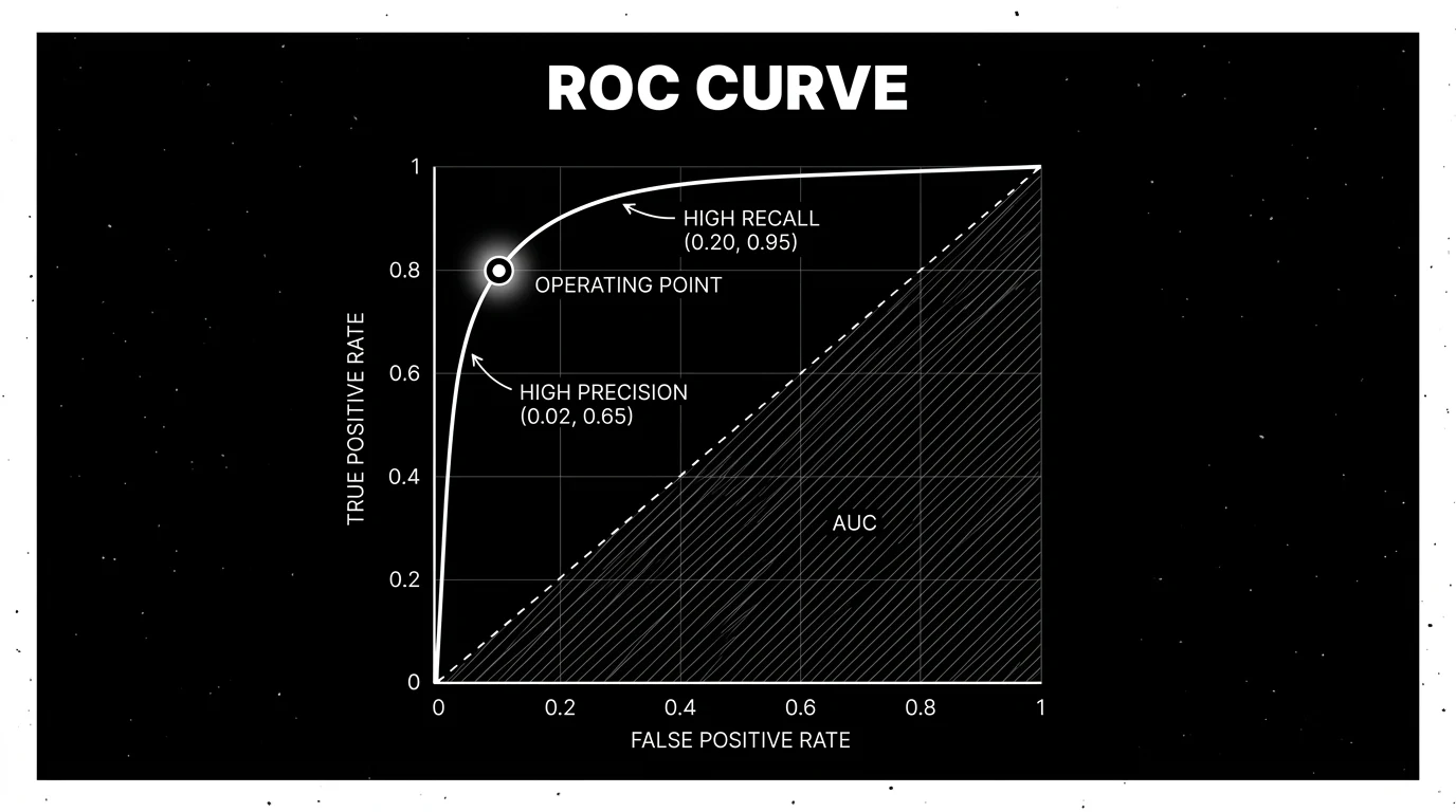
A good classifier hugs the upper-left corner: high TPR at low FPR. A bad classifier sits near the diagonal. Diagonal-equivalent AUC is 0.5; this is the random baseline.
The curve has structure beyond the AUC number. Two classifiers can have the same AUC and very different shapes:
- Curve dominates at low FPR. Useful for high-precision deployments where false alarms are expensive.
- Curve dominates at high recall. Useful for high-recall deployments where missed positives are expensive.
Compare models at the deployment operating region, not only by global AUC. The AUC summarizes the curve into one number; the curve shape is what tells you where the classifier is strong.
Operating points: where you actually deploy
The operating point is the threshold you commit to in production. It is one (FPR, TPR) pair on the curve. The operating point is the difference between a classifier that is “good in benchmark” and “deployed.”
Three patterns for picking the operating point:
Cost-curve method (most operationally honest)
Assign costs to false positives and false negatives. For a hallucination detector: a false positive (flagging a correct answer as hallucinated) might cost 1 unit (forces a re-read). A false negative (letting a hallucination through) might cost 50 units (user trust damage). Pick the threshold that minimizes expected cost = FP × cost_FP + FN × cost_FN.
Constraint method
Fix one of TPR or FPR at a business requirement, optimize the other. Examples:
- “We tolerate 2 percent false positive rate; what TPR can we reach?” Pick the threshold where FPR = 0.02.
- “We need to catch at least 95 percent of jailbreaks; what is the false-positive cost?” Pick the threshold where TPR = 0.95.
Youden’s J statistic
Maximize TPR - FPR across the curve. Simple, but treats false positives and false negatives as equally costly, which is rarely true.
A practical production scorecard publishes AUC-ROC, PR-AUC, and the chosen operating point with its TPR and FPR.
When AUC-ROC misleads
Three failure modes recur.
Severe class imbalance
Most LLM eval problems are imbalanced. Toxicity, jailbreaks, hallucinations, prompt injection, schema-violations: the positive class is 1 to 5 percent of traffic. AUC-ROC on imbalanced data can stay high while operational performance is poor. PR-AUC focuses on positive-class retrieval quality and makes low-base-rate false positives visible through precision, which is what users actually experience at low base rates.
A toy example: 99 negatives, 1 positive. A classifier that scores all negatives at 0.4 and the positive at 0.6 has AUC-ROC of 1.0 (perfect ranking). At threshold 0.5 it works. Add 10 negatives at score 0.7 (mistakes), and AUC-ROC drops to 0.91, but at the operating threshold of 0.5, the classifier now mis-flags 10 negatives for every 1 true positive. AUC was forgiving; precision-recall is not.
Cost asymmetry
If false negatives cost 50x more than false positives (or vice versa), the AUC summary across all thresholds buries the operating-point trade-off you care about. Always report the operating-point cost directly.
Comparing models with different score distributions
AUC-ROC is invariant to monotonic score transformations, but two classifiers can have the same AUC with very different score-to-probability mappings. One produces calibrated probabilities (a 0.7 score actually corresponds to 70 percent positive rate); the other does not. For LLM-judge applications where the score is read as a confidence, calibration matters and AUC alone misses it.
AUC-ROC for LLM-as-judge calibration
Applying AUC-ROC to LLM-judge evaluation:
- Build a labeled set. 200 to 1000 human-labeled examples on a binary good-vs-bad axis.
- Run the LLM-judge on each example, capturing a continuous score, or using a 1-to-5 rubric score as an ordinal ranking score.
- Plot ROC. TPR vs FPR across all judge thresholds.
- Compute AUC-ROC and PR-AUC.
- Pick the operating point based on cost or constraint.
In internal scorecards, teams often investigate calibration-set AUC-ROC below 0.75 before using a judge as a hard gate, and AUC-ROC of 0.95+ on a calibration set should trigger a sanity check (distribution mismatch between calibration and production traffic is a common cause). The acceptable threshold depends on task risk, class balance, label quality, and the cost of false positives versus false negatives.
For multi-rubric judges (factuality, helpfulness, fluency each scored separately), report AUC-ROC per rubric. Aggregate AUCs hide rubric-specific failures. See LLM-judge bias mitigation for the calibration pitfalls specific to LLM judges.
Calibration vs ranking
AUC-ROC measures ranking. It does not measure calibration directly. Two classifiers can have the same AUC but very different calibration:
- Classifier A produces calibrated probabilities (a 0.7 score corresponds to roughly 70 percent positive rate in the labeled set).
- Classifier B produces well-ranked but uncalibrated scores (a 0.7 score might correspond to 30 percent or 90 percent positive rate, depending on the threshold).
For deployment, calibrated probabilities matter. A 0.7 score that means “70 percent likely a hallucination” is more useful than a 0.7 that means “ranked higher than 70 percent of inputs.” Companion metrics: Brier score, log-loss, expected calibration error (ECE), and a calibration plot (actual positive rate vs predicted positive rate across score or probability bins). Our guide to evaluating LLM confidence and uncertainty goes deeper on calibration.
A practical scorecard for LLM-judges and detectors covers:
- AUC-ROC and PR-AUC.
- Operating point (TPR, FPR, precision, recall) at the deployment threshold.
- Calibration plot or ECE.
- Per-cohort breakdown (by intent, language, content type).
Common AUC-ROC mistakes
- Reporting AUC alone on imbalanced data. PR-AUC is the companion metric.
- Picking thresholds by Youden’s J without cost weighting. Treats FP and FN as equally costly when they almost never are.
- Comparing AUC across different test sets. Different distributions, different AUC, no apples-to-apples.
- Confusing AUC-ROC with calibration. Same AUC, different probability calibration.
- Reporting macro-AUC on multi-class without per-class. Aggregates hide class-specific failures.
- Using AUC-ROC as the only number on a production scorecard. It is one of three (AUC-ROC, PR-AUC, operating point) at minimum.
- Ignoring temporal drift. AUC measured at month one can be worse at month three; production reporting needs trend, not snapshot.
How to use this with FAGI
FutureAGI is the production-grade evaluation stack for teams calibrating LLM judges and detectors with AUC-ROC. The platform computes AUC-ROC and PR-AUC automatically when you score a labeled set against an LLM-judge or detector; ROC and PR curves render side by side, and the operating point is configurable per scorer. For continuous online calibration, the Agent Command Center routes a sample of production traces to human review, the new labels feed back into the AUC-ROC trend, and a drop in AUC against the calibration set triggers an alert. turing_flash runs guardrail-style screening at 50 to 70 ms p95; the heavier full eval templates run at roughly 1 to 2 second latency for offline calibration sets.
The same plane carries 50+ eval metrics, persona-driven simulation that produces calibration sets at scale, the BYOK gateway across 20+ providers via six native adapters (OpenAI, Anthropic, Gemini, Bedrock, Cohere, Azure) plus OpenAI-compatible presets and self-hosted backends, 18+ guardrails, and Apache 2.0 traceAI instrumentation on one self-hostable surface; pricing starts free with a 50 GB tracing tier. For benchmark continuity, scikit-learn’s roc_auc_score remains the standard implementation; FAGI eval templates wrap the same logic with span-attached scoring on production traces.
Sources
- scikit-learn ROC curve and AUC docs
- Fawcett (2006). An Introduction to ROC Analysis
- Saito and Rehmsmeier (2015). The Precision-Recall Plot Is More Informative than the ROC Plot
- Davis and Goadrich (2006). The Relationship Between Precision-Recall and ROC Curves
- Youden’s J statistic reference
- Liu et al. (2023). G-Eval: NLG Evaluation using GPT-4 with Better Human Alignment
Series cross-link
Related: F1 Score for Evaluating Classifiers, What is LLM Evaluation?, LLM-as-Judge Best Practices
Frequently asked questions
What is AUC-ROC in plain terms?
Why does AUC-ROC matter for LLM evals?
When does AUC-ROC mislead?
What is an operating point on the ROC curve?
How do I pick the operating point?
What is the difference between AUC-ROC and PR-AUC?
How does AUC-ROC apply to LLM-as-judge calibration?
Can AUC-ROC be used for multi-class LLM tasks?
Cost-efficient AI evaluation in 2026 is the cascade: classifiers, local heuristics, cheap judges. 7 platforms compared on per-eval cost.

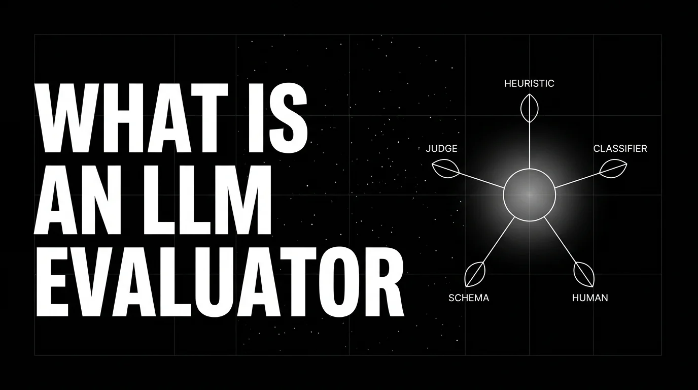
An LLM evaluator scores model outputs: heuristic, classifier, judge, programmatic, human. The 5 types, when each fits, and how to combine them in 2026.


LLM eval architecture in 2026: heuristics on every span, distilled judges on a sample, humans on the gold-set. Three-tier stack that scales.