Evaluating LLM Confidence and Uncertainty (2026): The Calibration Methodology
Logprob aggregation, semantic entropy, Brier score, and Platt scaling. The 2026 methodology for calibrated LLM confidence scores you can actually trust.
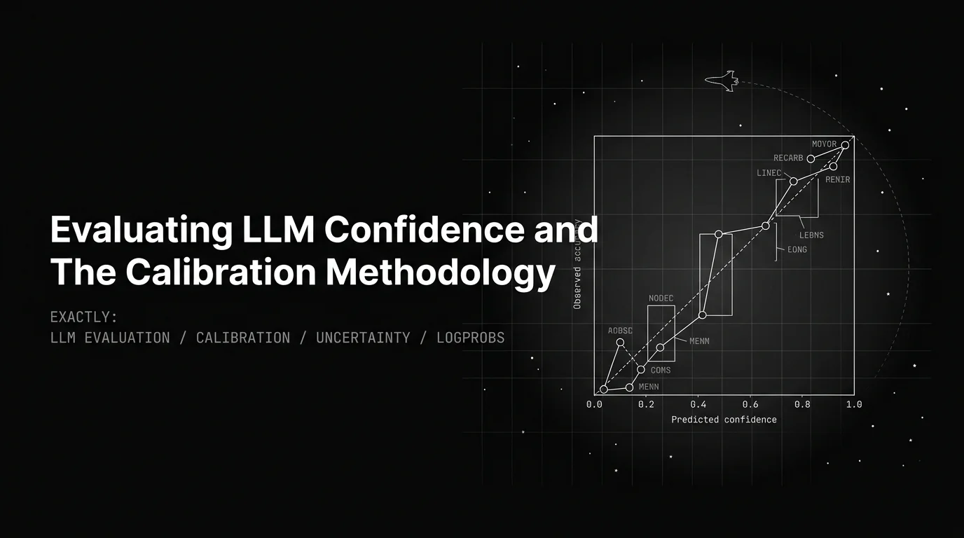
Table of Contents
An agent answers a customer question about prescription dosage. The model says it’s 0.92 confident. The answer is wrong. The customer follows the advice and ends up in the emergency room. The post-mortem reads like every other one: 0.9 verbalized confidence corresponded to 64% accuracy on the company’s labeled hold-out set. Nobody had measured calibration before launch. The escalation rule was “if confidence less than 0.5, escalate” — and the model almost never reported below 0.7.
LLM-stated confidence is theater. The model says “95% sure” and is wrong 30% of the time. The number is a generated token sequence, not an internal probability, and RLHF rewards the confident-sounding sequence over the hedged one. Teams that ship without measuring calibration get a uniform high-confidence stream that fails silently at the top of the curve.
The methodology that produces a confidence score you can actually trust has three legs: logprob aggregation when the provider exposes token probabilities, semantic entropy across paraphrase ensembles when it doesn’t, and Brier score against a held-out labeled set so you know how far the raw signal is from the truth. Without that triangulation, confidence is a number you don’t trust.
This guide covers each leg, the post-hoc calibration step (Platt scaling, isotonic regression) that maps a raw signal onto a usable probability, and the production patterns that put the whole loop on every span.
TL;DR: the calibrated confidence stack
| Signal | What it measures | When to use |
|---|---|---|
| Verbalized confidence | Model’s self-reported probability | One signal in an ensemble; never alone |
| Mean top-1 logprob | Average chosen-token probability over claim-bearing tokens | API exposes logprobs; structured or classification output |
| Top-k token entropy | Shannon entropy of next-token distribution | Same as above; high entropy flags hesitation |
| Semantic entropy | Entropy of meaning-clustered completions | API hides logprobs; open-ended generation |
| Brier score / ECE | Calibration gap on held-out labels | The metric that says how far off the raw signal is |
| Platt / isotonic | Post-hoc calibrator | Mapping raw signal to a usable probability |
| Classifier head | Trained on (input, was_correct) pairs | Workload-specific; highest accuracy with enough data |
The pipeline is the same shape every time. Collect a raw signal. Measure miscalibration on a held-out set. Fit a calibrator. Recalibrate when the distribution shifts.
Why verbalized confidence misleads
Three structural reasons the verbal number is biased.
Pretraining doesn’t teach calibration. The model is trained to predict the next token, not to predict whether the resulting answer is right. Internal token probabilities are well-calibrated for the next-token task. The verbal sentence “I’m 90% sure” is itself a sequence of tokens the model has chosen, conditioned on whatever pattern of confidence language showed up in training. It has no direct connection to the internal probability of the underlying claim.
RLHF amplifies overconfidence. Reward models prefer answers that sound decisive. The trained model learns that hedging is penalized in the reward signal, so it hedges less than it should. Tian et al. (2023) and follow-up work show that across GPT-4, Claude, and Llama-2 families, verbalized confidence is monotonically related to accuracy but systematically above the diagonal in the 0.7-1.0 region. The gap is largest exactly where it matters most: high-stakes high-confidence decisions.
Self-reports are post-hoc. Asking the model “how sure are you” generates a number after the answer is already on the page. The number is consistent with whatever rubric the prompt provided, not with an internal estimate of correctness. A different prompt produces a different scale.
The fix is not a better prompt. The fix is to replace the verbal number, or augment it, with a signal that has a defensible relationship to correctness. Two such signals are publicly available: logprobs and ensemble disagreement.
Logprob aggregation: when the API exposes them
OpenAI’s chat completions endpoint returns top-k log-probabilities when you pass logprobs=True. Most open-weight inference servers (vLLM, TGI, llama.cpp) expose them by default. Anthropic returns them on certain endpoints. When you can see logprobs, two derived signals dominate.
Mean top-1 logprob over claim-bearing tokens. Average the log-probability of the chosen token across the spans that carry semantic content (entities, numbers, names). Filler tokens (the, of, and) ride at near-1.0 probability regardless of correctness; including them washes out the signal. For structured outputs, restrict the aggregate to the parsed field tokens.
Top-k token entropy. Shannon entropy over the top-k token distribution at each step. High entropy means the model was choosing between several plausible tokens at that position. Spikes in entropy on claim tokens are strong correlates of error.
A working aggregator:
import math

def claim_token_uncertainty(tokens, claim_mask):
    # tokens: list of {token, top_logprob, top_k=[(tok, logp), ...]}
    # claim_mask: list of bool, True for claim-bearing positions
    logps, entropies = [], []
    for tok, is_claim in zip(tokens, claim_mask):
        if not is_claim:
            continue
        logps.append(tok["top_logprob"])
        probs = [math.exp(lp) for _, lp in tok["top_k"]]
        z = sum(probs)
        probs = [p / z for p in probs]
        entropies.append(-sum(p * math.log(p + 1e-12) for p in probs))
    return {
        "mean_logprob": sum(logps) / max(len(logps), 1),
        "mean_entropy": sum(entropies) / max(len(entropies), 1),
    }
Where logprob aggregation falls short: reasoning models. OpenAI’s o-series hides the chain-of-thought tokens. The visible logprobs cover the final-answer surface, which is often a confident summary of an internally uncertain reasoning trace. Same pattern for any model behind a “reasoning” or “thinking” wrapper. Treat logprob aggregation as one signal for these models, not the primary one.
Semantic entropy: when logprobs are hidden
For any API that hides logprobs (most hosted commercial endpoints in 2026), the workaround is to estimate uncertainty from sampling behavior. The naive version is lexical entropy: sample N completions at temperature 0.7 and measure how often the surface strings agree. The problem is that paraphrases register as disagreement: “Paris is the capital” and “The capital is Paris” look distinct lexically while expressing the same answer.
Semantic entropy (Farquhar et al., Nature 2024) fixes this. Sample N completions, cluster them by meaning, and compute entropy over the cluster proportions instead of the raw strings. Two ways to cluster:
- Bidirectional NLI. Two completions belong in the same cluster if a small NLI model says each entails the other. Computationally heavier, more accurate on paraphrase-heavy tasks.
- Embedding then cluster. Embed each sample with a sentence encoder; cluster with HDBSCAN or agglomerative clustering at a tuned threshold. Cheaper, looser on edge cases.
A reference implementation:
import math
from collections import Counter

def semantic_entropy(samples, equivalent_fn):
    # samples: list of generated strings
    # equivalent_fn(a, b) -> bool: bidirectional NLI or embedding-distance check
    clusters = []
    for s in samples:
        placed = False
        for cluster in clusters:
            if equivalent_fn(s, cluster[0]):
                cluster.append(s)
                placed = True
                break
        if not placed:
            clusters.append([s])
    n = len(samples)
    probs = [len(c) / n for c in clusters]
    return -sum(p * math.log(p + 1e-12) for p in probs)
Farquhar et al. report semantic entropy detecting hallucinations 10 to 15 points more accurately than lexical entropy or verbalized confidence across question-answering benchmarks. The cost is the N samples. For an agent at 50 calls per second with N=5, the inference cost is 5x baseline. Route only the high-stakes calls through it. The Agent Command Center makes the cost auditable per call via agentcc_cost_total and agentcc_tokens_total Prometheus counters.
Where semantic entropy falls short: tasks where multiple correct answers exist (open-ended generation, creative tasks). Entropy is high because the answer space is large, not because the model is uncertain. Anchor the metric on tasks with a defensible ground truth.
Brier score, ECE, and the reliability diagram
A raw signal is useful only if you know how miscalibrated it is. The headline metric is Brier score: the mean squared error between predicted probability p_i and the binary correctness label y_i, averaged over N samples. Lower is better. Brier decomposes into a calibration term (how close binned predictions are to observed accuracy) and a sharpness term (how often the model commits to extreme probabilities versus sitting at 0.5). A constantly-0.5 model has perfect calibration on a 50/50 task and terrible sharpness; you want both.
Expected Calibration Error (ECE) is the binned reliability gap: split predictions into B confidence bins (10 is standard), compute the absolute gap between the bin’s observed accuracy and its mean predicted probability, and take the sample-weighted average across bins. ECE below 0.05 on your labeled set is a reasonable production target.
The reliability diagram is the picture both metrics summarize: predicted confidence on the x-axis, observed accuracy on the y-axis, one point per bin. A well-calibrated signal sits on the diagonal. Most off-the-shelf LLMs sit well above it in the 0.7-1.0 region — over-confident, exactly as RLHF predicts. For the related operating-point view on classifier-style evals, see AUC-ROC for LLM evals.
Compute all three on a held-out labeled set of 500 to 2000 production-representative examples. Pull traces from production, not invented test cases. Skew toward the hardest 10% of inputs (edge cases, rare intents). Label by hand. This is the gold-set; everything downstream depends on it. The synthetic test data guide covers how to scale labeled coverage without losing signal.
Calibration: Platt scaling and isotonic regression
The raw signal (verbalized, logprob mean, semantic entropy) is rarely calibrated out of the box. Two standard post-hoc fixes turn a miscalibrated signal into a usable probability.
Platt scaling fits a one-parameter logistic regression on (raw_signal, was_correct) pairs from a calibration split:
import numpy as np
from sklearn.linear_model import LogisticRegression

def fit_platt(raw_signals, labels):
    X = np.array(raw_signals).reshape(-1, 1)
    y = np.array(labels)
    return LogisticRegression().fit(X, y)

def apply_platt(model, raw_signal):
    return model.predict_proba([[raw_signal]])[0, 1]
Works well when miscalibration is monotonic and roughly linear in logit space. Cheap to fit, stable on small calibration sets (200+ examples), the default starting point.
Isotonic regression fits a non-parametric monotonic mapping. Handles weirder calibration curves where the bias is non-linear:
from sklearn.isotonic import IsotonicRegression

def fit_isotonic(raw_signals, labels):
    return IsotonicRegression(out_of_bounds="clip").fit(raw_signals, labels)
Needs more data (1000+ examples for stability) but reads off the data without parametric assumptions. The right choice when Platt under-corrects in the tails.
Fit on a calibration split. Validate on a held-out test split. Check that Brier and ECE actually improve (they usually do — Platt scaling commonly cuts ECE by 30 to 60 percent on verbalized confidence). Then deploy the calibrator as a thin wrapper on the raw signal.
Recalibrate when the model version changes, when the prompt template changes substantively, or when the input distribution shifts. The calibrator is a contract between the model and the production traffic; the contract breaks when either side moves.
Production patterns
Three pieces wire the whole loop into production. Span instrumentation that captures the raw signals, a labeled set that anchors calibration, and a gate that routes uncertain answers to escalation.
Instrumentation with traceAI
traceAI (Apache 2.0, OpenTelemetry-native) captures confidence signals as custom span attributes alongside the standard OTel GenAI fields. Auto-instrumentation across OpenAI, LangChain, Groq, Portkey, and Gemini means the LLM span exists; you only have to add the uncertainty attributes.
from fi_instrumentation import register
from fi_instrumentation.fi_types import ProjectType
from traceai_openai import OpenAIInstrumentor
from opentelemetry import trace

trace_provider = register(
    project_type=ProjectType.OBSERVE,
    project_name="confidence-eval",
)
OpenAIInstrumentor().instrument(tracer_provider=trace_provider)

tracer = trace.get_tracer(__name__)

def answer_with_uncertainty(prompt, n_samples=5):
    with tracer.start_as_current_span("llm.answer_with_uncertainty") as span:
        samples = [
            client.chat.completions.create(
                model="gpt-4.1",
                messages=[{"role": "user", "content": prompt}],
                temperature=0.7,
                logprobs=True,
                top_logprobs=5,
            )
            for _ in range(n_samples)
        ]
        sem_entropy = semantic_entropy(
            [s.choices[0].message.content for s in samples],
            equivalent_fn=nli_equivalent,
        )
        logp_signal = claim_token_uncertainty(
            extract_tokens(samples[0]),
            claim_mask=mask_claims(samples[0]),
        )
        span.set_attribute("llm.semantic_entropy", sem_entropy)
        span.set_attribute("llm.mean_top_logprob", logp_signal["mean_logprob"])
        span.set_attribute("llm.mean_entropy", logp_signal["mean_entropy"])
        span.set_attribute("llm.n_samples", n_samples)
        return majority_answer(samples), sem_entropy, logp_signal
The three custom attributes ride the trace tree. Pluggable semantic conventions (FI, OTEL_GENAI, OPENINFERENCE, OPENLLMETRY) at register() time mean the same trace ingests cleanly into Phoenix or Traceloop without re-instrumenting.
Evaluating against the labeled set
The ai-evaluation SDK (Apache 2.0) ships the rubric surface. AnswerRefusal, TaskCompletion, and Groundedness are three of the 60+ EvalTemplate classes that map directly to “did the agent escalate when it should” and “was the answer correct against context.” CustomLLMJudge is the authoring primitive for calibration-specific rubrics on top of those.
from fi.evals import Evaluator
from fi.evals.templates import AnswerRefusal, TaskCompletion, Groundedness
from fi.evals.metrics import CustomLLMJudge
from fi.evals.llm.providers.litellm import LiteLLMProvider
from fi.testcases import TestCase

evaluator = Evaluator(fi_api_key=..., fi_secret_key=...)

calibration_judge = CustomLLMJudge(
    provider=LiteLLMProvider(),
    config={
        "name": "CalibrationScore",
        "model": "gpt-4.1",
        "grading_criteria": """Given the input, the agent's answer, and the
stated confidence (0-1), return 1.0 if confidence above 0.7 and answer correct,
or confidence below 0.3 and answer wrong. Return 0.0 if confidence above 0.7
and answer wrong (over-confident wrong).""",
    },
)

results = evaluator.evaluate(
    eval_templates=[AnswerRefusal(), TaskCompletion(), Groundedness(), calibration_judge],
    inputs=[
        TestCase(
            input=row.input,
            output=row.output,
            context=row.context,
            metadata={
                "stated_confidence": row.stated_confidence,
                "was_correct": row.was_correct,
            },
        )
        for row in labeled_set
    ],
)
The Platform’s self-improving evaluators retune from production thumbs feedback at lower per-eval cost than Galileo Luna-2, so the calibration rubric ages with the product instead of drifting against last quarter’s distribution.
Deploying the uncertainty gate
A calibrated probability becomes an operating threshold. The threshold is a business decision (medical triage operates at a different point on the curve than internal chat); the calibration is engineering.
def route(prompt):
    answer, sem_ent, logp = answer_with_uncertainty(prompt)
    raw = combine(sem_ent, logp["mean_logprob"], verbalized_confidence(answer))
    p_correct = platt.predict(raw)  # calibrated probability
    if p_correct < 0.65:
        return escalate_to_human(prompt, reason=f"p_correct={p_correct:.2f}")
    return answer
Error Feed clusters the failures via HDBSCAN soft-clustering over ClickHouse-stored embeddings. A Sonnet 4.5 Judge agent writes the immediate_fix per cluster against a 5-category 30-subtype taxonomy. The fixes feed back into the Platform’s self-improving evaluators so calibration drift surfaces as a specific recurring failure mode, not a vague score that moved.
Where Future AGI’s eval stack fits
Three surfaces, one story.
- ai-evaluation SDK (Apache 2.0). 60+
EvalTemplateclasses coveringAnswerRefusal,TaskCompletion,Groundedness, plus 20+ local heuristic metrics (BLEU, ROUGE, JSON schema, embedding similarity) at sub-10 ms with zero API cost.CustomLLMJudgeis the authoring primitive forCalibrationScore,HedgeLanguageQuality, and any workload-specific calibration rubric. - Future AGI Platform. Self-improving evaluators retune from production thumbs feedback, classifier-backed scoring at lower per-eval cost than Galileo Luna-2, in-product agent authoring for the calibration loop. The threshold-tuning loop closes without re-authoring rubrics.
- Error Feed (inside the eval stack). HDBSCAN over ClickHouse, Sonnet 4.5 Judge writes
immediate_fixper cluster against the 5-category 30-subtype taxonomy. Linear ships today as the only routed integration.
traceAI (Apache 2.0) ships 50+ AI surfaces across four languages with auto-instrumentation on OpenAI, LangChain, Groq, Portkey, and Gemini. The Agent Command Center is the SOC 2 Type II, HIPAA, GDPR, and CCPA certified hosted runtime per futureagi.com/trust, with 100+ providers, 18+ built-in guardrail scanners plus 15 third-party adapters, and agentcc_cost_total / agentcc_tokens_total Prometheus counters that make the N-sample semantic entropy cost auditable per call.
Ready to put calibrated confidence under your own workload? Start with the ai-evaluation SDK quickstart, instrument logprobs and semantic entropy on your LLM spans via traceAI, and fit a Platt calibrator on a 500-example labeled set this week. The calibrated probability is the artifact — not the verbal number the model generated.
Three takeaways for 2026
- Verbalized confidence is one signal, never the primary one. Logprob aggregation when the API exposes them, semantic entropy when it doesn’t. Combine.
- Brier score and ECE on a held-out labeled set are the contract. Without the labeled set, you don’t know how far off the raw signal is, and threshold tuning is hopeless.
- Post-hoc calibration is cheap, and you have to recalibrate. Platt scaling on 200+ examples will commonly cut ECE by 30 to 60 percent on verbalized confidence. Refit when the model, prompt, or distribution shifts.
Related reading
- The 2026 LLM Evaluation Playbook
- LLM-as-Judge Best Practices (2026)
- Your Agent Passes Evals and Fails in Production (2026)
- Deterministic LLM Evaluation Metrics (2026)
- Detect Hallucinations in Generative AI
- LLM Tool Chaining and Cascading Failures
Sources
- Farquhar, S. et al. “Detecting hallucinations in large language models using semantic entropy.” Nature (2024).
- Tian, K. et al. “Just Ask for Calibration: Strategies for Eliciting Calibrated Confidence Scores from Language Models Fine-Tuned with Human Feedback.” EMNLP (2023).
- Future AGI ai-evaluation SDK
- Future AGI traceAI SDK
- Future AGI Agent Command Center docs
- Future AGI trust center
Frequently asked questions
Why is verbalized LLM confidence unreliable?
What is semantic entropy and when do I use it?
What is Brier score and why is it the right calibration metric?
How do I calibrate an LLM's confidence after measuring miscalibration?
Should I always use logprob aggregation when it's available?
How does Future AGI fit into a confidence evaluation workflow?
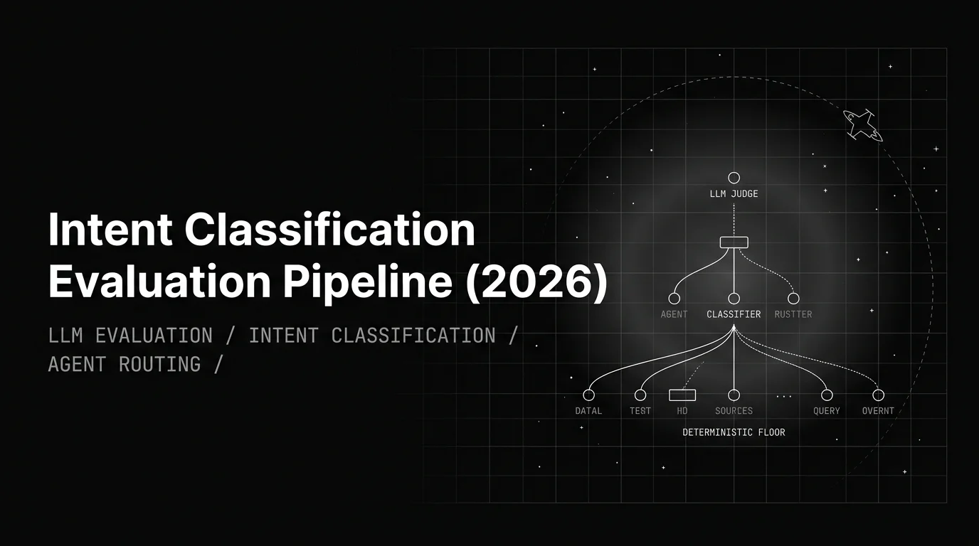
Per-intent precision-recall, escalation accuracy, OOD detection, and drift gates for the LLM router that decides which pipeline runs.

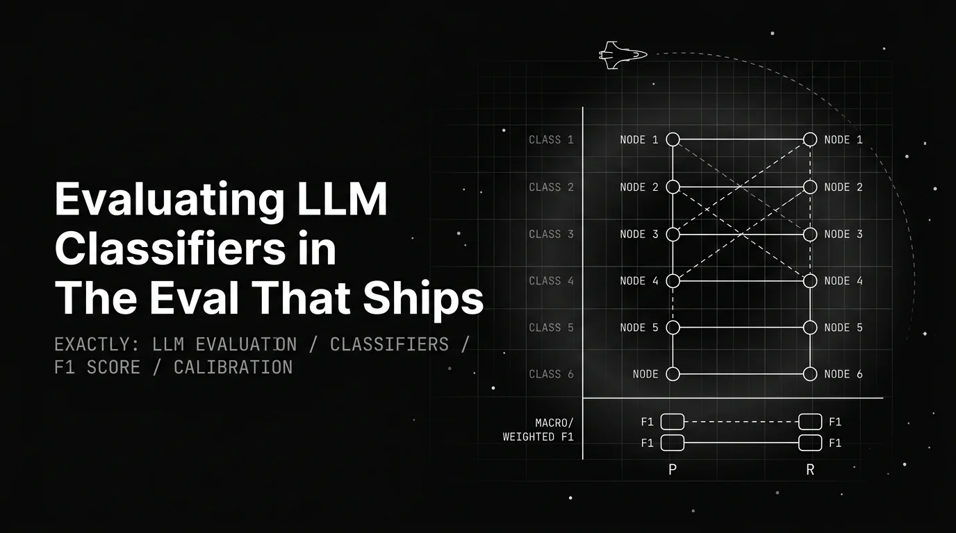
Evaluating LLM classifiers in 2026: per-class precision-recall, macro vs weighted F1, production-distribution calibration, confusion-matrix debugging.


Literal AI's hosted platform was discontinued. This migration guide ranks five alternatives and shows how to move traces, datasets, and prompts off it.