How to Benchmark a Vector Database: The Three Numbers That Decide It
Published vector database benchmarks do not transfer to your corpus. Measure three numbers yourself: recall at your k, pgvector index build cost, and filtered p95.
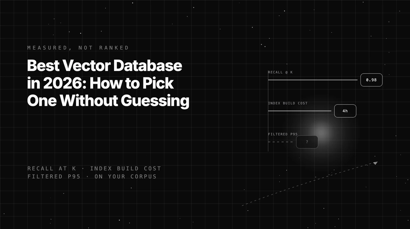
Table of Contents
You have embeddings, a corpus, and a migration you are about to justify. What you do not have is a vector database benchmark that was run on your data.
That is the whole problem with the published ones. They measure recall and queries per second on public embedding sets, at dimensions you are not using, with query distributions that are not yours, and almost none of them apply a filter. Then a leaderboard gets built on top of those numbers and circulated as though it settles something.
It does not, because the three numbers that actually decide this depend on your corpus rather than on the product. This post is the procedure for getting them: the SQL to run, the parameters to record, and the one number the entire category leaves out. It is written against pgvector, since that is where most projects start and where the sharpest surprises live, but the method transfers.
If what you want is the store-by-store comparison rather than the measurement procedure, read best vector databases for RAG instead.
What Does a Vector Database Do That a Library Does Not?
Worth settling first, because a portion of readers are about to add infrastructure they do not need.
The index is the interesting part
An approximate nearest neighbour index (HNSW, IVF, DiskANN and their variants) trades exact results for a search that does not have to touch every vector. Instead of comparing your query against the whole corpus, it navigates a structure that gets you close, usually very close, while looking at a fraction of the data. That trade is the entire reason any of this exists, and it is why “recall” is a number you have to think about at all.
The database is everything wrapped around the index
FAISS gives you an index, and it will serialise that index to a file. What it does not give you is transactional durability, metadata filters that stay consistent with the index as rows change, replication, concurrent writers, or multi-tenancy. A vector database is an ANN index plus the operational surface that lets more than one process depend on it.
Framed that way, the question “do I need a vector database” becomes answerable. If a single process loads a static index at startup and nothing writes to it, you need a library. If several services read while something writes, you need a database.
This post is about picking that database. If the question you actually have is whether to retrieve by vector similarity or by graph traversal, that is a different decision, covered in Vector Databases and Knowledge Graphs for RAG.
The Three Numbers Your Vector Database Benchmark Has to Produce
Here is what actually separates one choice from another once the feature lists have cancelled out. Two of the three are well-trodden and we have written them up elsewhere. The third is the one nobody publishes, so it gets the most room here.
Recall at your k, on your corpus
Public benchmarks measure recall on public embedding sets. Your recall depends on your embedding model, chunk size, dimensionality and query distribution, and the benchmark shares none of those. A store that wins on a standard dataset can lose on yours.
The short version of the method: sample two to five hundred real queries from your logs, compute
exact top-k by brute force offline, and measure what the index returns against that ground truth.
One caveat matters more than the store you picked. Recall is a function of index parameters, not
just index type, so two teams reporting different recall for the same database are usually reporting
different points on the same curve. Record m, ef_construction and ef_search next to every
number or the number expires.
The full protocol, including how to build exact-knn ground truth and how to read p99 under filter cardinality, is in Evaluating Vector Database Recall Quality. This post will not re-derive it.
Index build cost at your row count
This is the number that decides migrations and the one the comparison posts leave out. Among the comparison posts we checked, we did not find one that reports a measured index build time or peak build memory for any store; the closest any comes is repeating a vendor’s relative indexing-speed claim. It is also the number most likely to break a deployment plan, because unlike recall it is a hard operational constraint with a wall clock attached to it.
HNSW builds have to hold the graph in memory while constructing it. In Postgres, the parameter that
governs this is maintenance_work_mem, which
defaults to 64 MB. Set it
too low for your row count and the build does not fail. It spills to disk and gets dramatically
slower, and pgvector tells you so in a notice that almost never gets read in build logs:
NOTICE:  hnsw graph no longer fits into maintenance_work_mem after 100000 tuples
DETAIL:  Building will take significantly more time.
HINT:  Increase maintenance_work_mem to speed up builds.
Teams discover this when a build they expected to take twenty minutes is still running the next morning.
Raise maintenance_work_mem for the build itself, and increase
max_parallel_maintenance_workers so the build uses more than one core. See the
pgvector index build notes and
ClickHouse’s guide to scaling pgvector,
which recommends values in the 8 GB to 16 GB range for large builds on suitably sized instances.
Run this against your own corpus. It is the whole measurement, and it takes one build cycle:
-- 1. Size the build. Watch for the NOTICE above in your logs.
SET maintenance_work_mem = '8GB';
SET max_parallel_maintenance_workers = 7;  -- plus the leader
SET client_min_messages = 'notice';

-- 2. Cold build over the full corpus, timed.
\timing on
CREATE INDEX CONCURRENTLY items_embedding_hnsw
  ON items USING hnsw (embedding vector_cosine_ops)
  WITH (m = 16, ef_construction = 64);
\timing off

-- 3. What it cost you on disk.
SELECT pg_size_pretty(pg_relation_size('items_embedding_hnsw')) AS index_size,
       pg_size_pretty(pg_relation_size('items'))                AS table_size;
Record wall time, peak memory and index size, and record m and ef_construction beside them.
Raising ef_construction buys recall and costs build time, so a build number without its parameters
is not comparable to anything, including your own next run.
The constraint that catches teams before any of this is dimensionality. pgvector’s vector type
indexes up to 2,000 dimensions, with halfvec reaching
4,000 and binary quantization 64,000. A 3,072-dimension embedding stores fine and then fails at
CREATE INDEX, which is a late and expensive place to discover it. Check this before you pick the
embedding model, not after.
Measure two things: wall time for a cold build of your full corpus, and peak memory during it. If the build does not fit inside your maintenance window, that is a hard constraint no feature list will warn you about.
Filtered query latency
Unfiltered queries per second is the number vendors publish. It is also the number nobody runs in production, because production queries almost always carry a filter: this tenant, this document set, this date range, this language.
Where the store applies the filter changes the answer completely, and the three engines people actually shortlist do three different things.
pgvector post-filters: it scans the index, then applies the WHERE clause to what came back. Its
own documentation is blunt about the consequence. With the default hnsw.ef_search of 40, a
condition matching 10% of rows leaves about four results. The query does not slow down, it silently
under-returns.
Since 0.8 you can set hnsw.iterative_scan to keep scanning until enough rows survive the filter,
bounded by hnsw.max_scan_tuples (20,000 by default). That buys recall back and spends tail latency
and CPU to do it:
SET hnsw.iterative_scan = relaxed_order;  -- or strict_order for exact distance ordering
SET hnsw.max_scan_tuples = 20000;

EXPLAIN ANALYZE
SELECT id FROM items
WHERE tenant_id = 42
ORDER BY embedding <=> $1
LIMIT 10;
Run that with and without the filter, and with iterative_scan off and on. Four numbers, one
session, and they tell you whether your store is silently under-returning today. Source:
pgvector on filtering and iterative index scans.
Milvus goes the other way and restricts the search scope to entities matching the filter before searching. Qdrant does neither: it extends the HNSW graph with edges built from indexed payload values and uses filter-cardinality estimates to choose between traversing that graph and falling back to a full scan.
The practical consequence is that a highly selective filter is the case where the ANN index stops earning its place. At that end, an exact B-tree index on the filter column, a partial index, or partitioning usually beats the graph, which is what pgvector’s own docs recommend for conditions matching a low percentage of rows.
Measure p50 and p95 with your real filter, not without it, and record which mechanism your store is using when you do.
What to Benchmark Against, and When Not to Bother
Before you spend an afternoon measuring, it is worth knowing which comparison is even worth setting up. Some situations are decided by architecture rather than by numbers, and benchmarking them is effort you will not get back. If what you want is the store-by-store breakdown rather than the measurement procedure, Best Vector Databases for RAG: 7 Stores Compared takes Pinecone, Milvus, Weaviate, Qdrant, pgvector, Chroma and Vespa one at a time.
| Your situation | Reasonable choice | The reason |
|---|---|---|
| Already run Postgres, single-node corpus | pgvector | One database, one backup story, SQL joins between vectors and metadata |
| Want zero operational work and will pay for it | A managed service | You are buying the absence of an on-call rotation, not better recall |
| Corpus outgrows one node, dedicated team | A distributed engine such as Milvus | pgvector has no built-in sharding; you add Citus or PgDog to get it |
| Latency-sensitive with heavy metadata filtering | An engine with filter-aware indexing, such as Qdrant | Filtering strategy dominates at this profile |
| Prototyping, corpus fits in memory, no concurrent writes | An embedded store or a library | A server is operational overhead with no payoff yet |
| Under a hundred thousand chunks | Brute force in whatever you already have | Exact search, no index, no tuning, no drift |
Two warnings about this table. It reflects positioning and architecture rather than benchmark results, and it is deliberately not a ranking. Before you commit to any row, confirm the current licence, hosting model and index support directly from that vendor’s own documentation, because in this category those change often enough that a table written today can mislead by next quarter.
Why Your Existing Postgres Is Probably the Right Default
The strongest argument for pgvector is not performance. It is that vectors and the metadata you filter on live in the same database, so a query that says “the ten nearest chunks belonging to this tenant, from documents published this year, excluding archived ones” is one SQL statement against one consistent snapshot.
Split those across two systems and you inherit a synchronisation problem that nobody puts in the comparison table. The document gets deleted in Postgres and the embedding lingers in the vector store. Now your retrieval returns a chunk from a document that no longer exists, and your generator answers from it.
The honest limit is that there is no single row count at which pgvector stops working. ClickHouse’s guide to scaling pgvector describes bands rather than a cliff. Naive setups usually hold around a million vectors. Quantization and strict memory tuning start to matter well before ten million. A pure Postgres architecture stops being the simplest answer once you are past a billion, or need sub-20ms p99 under heavy concurrency.
What moves those bands is dimensionality, hardware, recall target and filter pattern. Treat any number you read as a starting hypothesis rather than a specification, including ours.
The structural limit is cleaner than the performance one. ParadeDB notes that native sharding of vector data across nodes is not supported, and that HNSW indexes do not reclaim space when rows are deleted. Tombstoned nodes stay in the graph until the index is rebuilt, so if your corpus turns over constantly, budget for the rebuild.
There is a second cost to the split that shows up later. Two systems means two consistency models, two failure modes during deploys, and two places where a backfill can go half-finished. The failure is rarely dramatic. It is a slow divergence where a few thousand rows drift out of sync during an incident and nobody notices for a month, because retrieval degrading by two percent does not page anyone. Single-store setups get this for free, which is a real operational property even though it never appears in a benchmark.
The point is not that pgvector wins. It is that the burden of proof sits with the migration. Adding a second database has a known cost and an unknown benefit until you measure.
When the Benchmark Is Not Worth Running at All
Three cases where the answer is no, and all three are more common than the market implies.
Your corpus is small. Our rule of thumb, not a measured constant: under roughly a hundred thousand chunks at typical embedding dimensions, exhaustive search over a matrix is fast enough for interactive use and it is exact, so recall stops being a thing you have to think about. Check it against your own hardware and latency budget. Every ANN index is an optimisation you have not yet earned.
Your corpus is static and single-process. If the index is built once, loaded at startup and never written to, you want a library and a file. The database features are all about coordination you do not need.
Your retrieval problem is not actually semantic. This one is worth checking before anything else. Run BM25 or plain keyword search over your corpus and measure. If lexical search already answers most of your queries acceptably, embeddings are not your bottleneck and a vector database will not become one. Hybrid retrieval exists precisely because the two catch different failures.
The Measurement Plan You Run Before You Commit
Five tests, one afternoon, before any migration.
Scope, so you can judge what follows: the SQL and parameter defaults here describe pgvector 0.8 or later, read from the pgvector and PostgreSQL documentation and last verified on 6 August 2026. Confirm them against your own installed version, since defaults move between releases. The commands are a harness for you to run, not results we are reporting. We have deliberately not published our own numbers, because a benchmark on our corpus would be exactly the kind of number this post argues you should ignore.
| Test | What you run | What you record | Pass condition |
|---|---|---|---|
| Recall | 300 sampled production queries against brute-force ground truth | recall@10 | Within your tolerance of exact |
| Build | Cold index build over the full corpus | Wall time, peak memory | Fits your maintenance window |
| Filtered latency | The same queries with your real production filter | p50, p95 | p95 inside your latency budget |
| Write path | Sustained upserts while querying | Query p95 during writes | No collapse under concurrent load |
| Exit | Dump vectors plus metadata to a portable format | Wall time, fidelity | Completes, nothing lost |
The exit row is the one people skip and the one that matters most, because it is the only test that prices the risk of being wrong. A store you can leave in an afternoon is a reversible decision. A store you cannot is a commitment you are making on the strength of a benchmark you did not run.
The recall row is the only one that needs code rather than SQL, because ground truth has to come from exhaustive search:
import numpy as np

def recall_at_k(index_results, corpus, queries, k=10):
    """index_results[i] = ids the store returned for queries[i]."""
    hits = 0
    for q, returned in zip(queries, index_results):
        # Exact top-k by brute force. Slow, and that is fine offline.
        exact = np.argsort(-(corpus @ q))[:k]
        hits += len(set(exact) & set(returned[:k]))
    return hits / (k * len(queries))
Normalise your vectors first if you are measuring cosine similarity, and sample the queries from production logs rather than writing them, because invented queries are more uniform than real ones and will flatter the index.
There is one more gap worth naming before you finish. Recall measures what came back from the index. It says nothing about whether the generator used it. You can hit recall@10 of 0.98 and still ship a wrong answer, because the model had the right chunks in context and answered from something else. Retrieval quality and answer quality are different measurements, and only one of them is the one your users experience.
Where Future AGI Fits
That last gap is what Future AGI’s retrieval evaluation templates are for. They ship in the open-source Future AGI platform, which is Apache-2.0 and self-hostable, and are documented in the built-in evals reference.
context_relevance is an
LLM-as-judge eval that reads the query and the retrieved context and scores how relevant and
sufficient that context is for answering the question. Sufficiency is the half that matters here:
the index can return the right document and still not return enough of it.
chunk_attribution
returns a single Pass or Fail for whether the output shows the model drew on the retrieved context
at all. This is the generator’s side of the problem. If you need to know how much of the context
was used rather than whether any of it was, that is a separate eval,
chunk_utilization.
Both run the same way, against the context your store actually returned:
from fi.evals import evaluate

result = evaluate(
    "context_relevance",
    input=query,
    context=retrieved_chunks,
    model="turing_flash",
)
print(result.score, result.reason)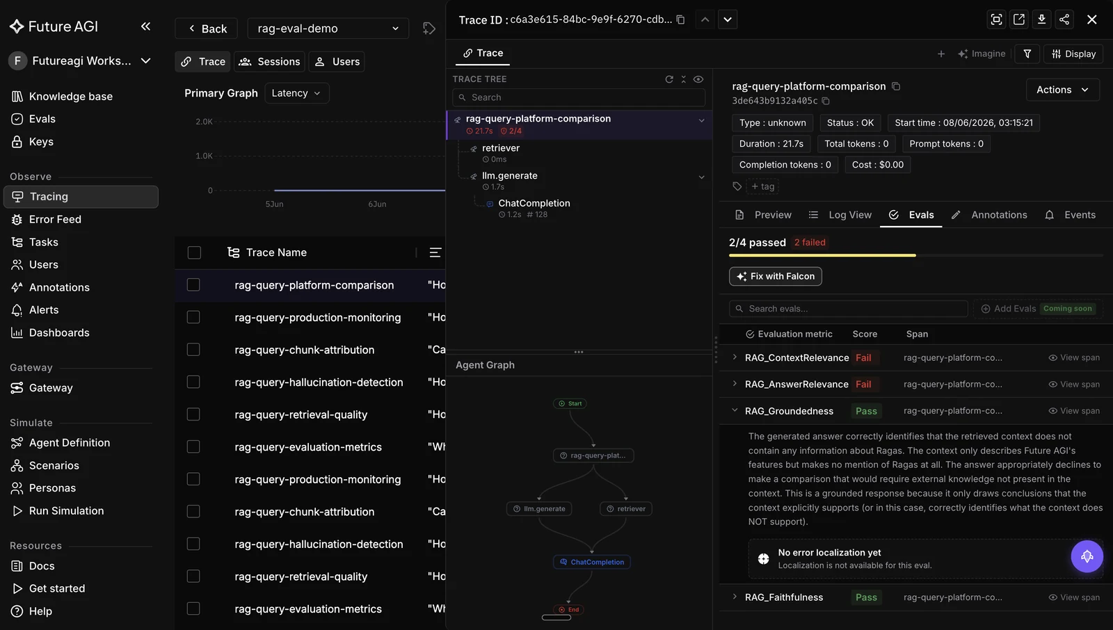
The screenshot above is the shape of the diagnosis. The trace view labels evals by display name, so
the template you call context_relevance from the SDK appears there as RAG_ContextRelevance.
Context relevance has failed while groundedness has passed, which reads as retrieval returned the wrong material and the generator correctly refused to invent around it. That is a retrieval problem, and it is the case where changing stores or tuning index parameters is worth your time. Flip the two results and you have the opposite conclusion.
Both scores attach to the span that produced them, so the retriever span carries the retrieval verdict rather than leaving you to infer it from the final answer.
Run together, they separate two failures that look identical from the outside. If
context_relevance is low, your retrieval is the problem and a different vector database might
genuinely help. If context_relevance is high and chunk_attribution shows the model ignoring
what it was given, changing stores will not move anything, because the fault is in the prompt or the
generation step.
That distinction is worth having before a migration, not after one.
Neither template is something you configure from scratch. They sit in the evals catalog alongside the rest, filterable by the RAG and Retrieval Systems tags.
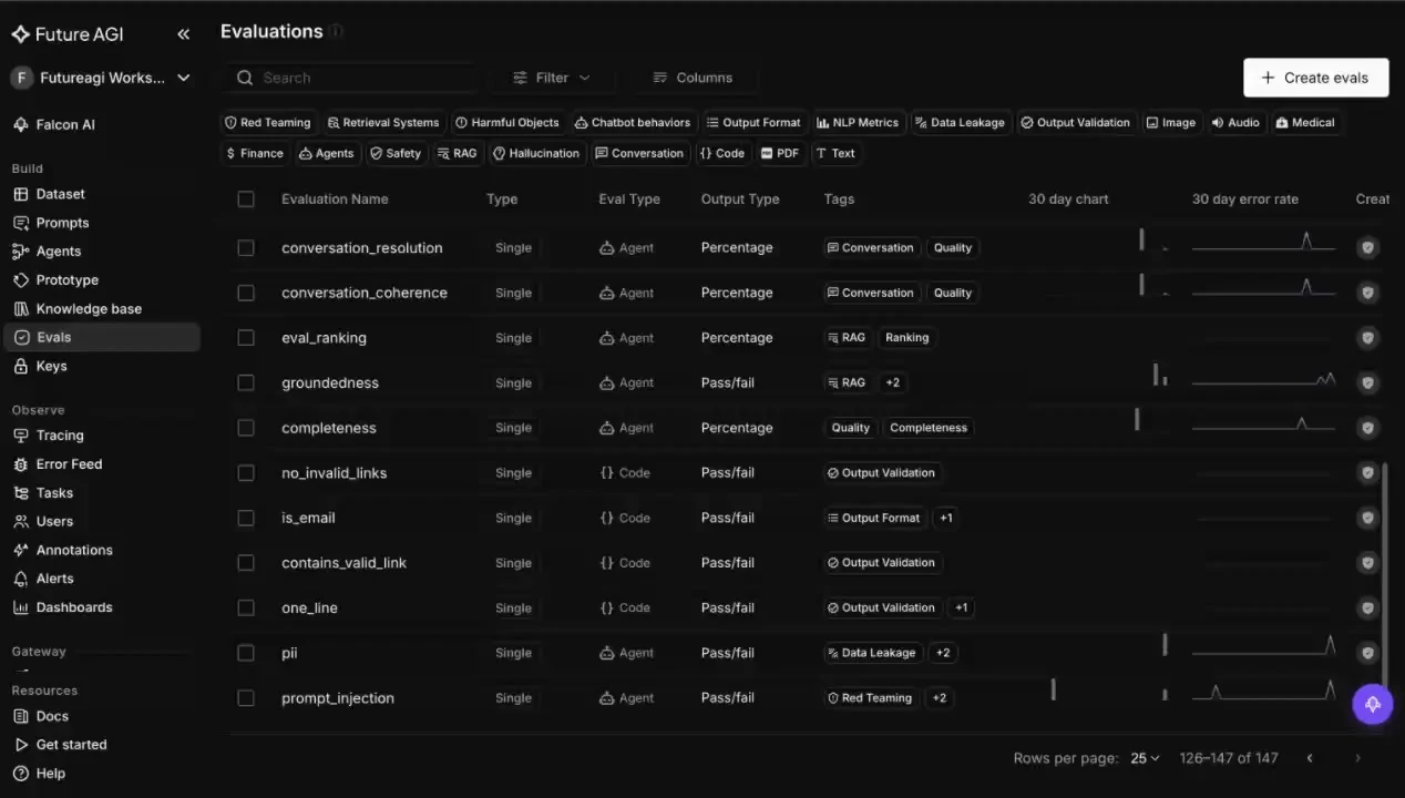
The 30 day error rate column on the right of that catalog is the part worth noticing for this post. Once a retrieval eval is running, its failure rate becomes a time series, which means a change in chunking, embedding model or index parameters shows up as a movement you can attribute rather than a regression someone reports in three weeks.
Conclusion
The shortlist is not the deliverable. The benchmark you ran yourself is.
Recall at your k, index build cost at your row count, filtered p95 with your real filter. Three numbers, measured on your corpus, in an afternoon. Every leaderboard you have read is an argument about a corpus that is not yours.
If you run only one of the three, run the build. It is the number no comparison post publishes, it is the one that turns into a missed maintenance window rather than a slightly worse answer, and it is the one you cannot discover late without paying for it twice.
Start from what you already run, make the migration prove itself, and test whether you can leave before you commit to arriving.
Want to measure retrieval quality before you migrate? Start in the Future AGI app and
follow the evaluation docs to run context_relevance and chunk_attribution against
your own corpus. The platform is open source at future-agi/future-agi.
Frequently Asked Questions
How do I benchmark a vector database?
What limits pgvector performance in production?
What is the difference between a vector database and a vector index?
Why do published vector database benchmarks not transfer?
Do I need a vector database for a small corpus?
Pinecone, Milvus, Weaviate, Qdrant, pgvector, Chroma, Vespa for RAG in 2026. Compared on recall, latency, hybrid search, OSS license, eval-fit.

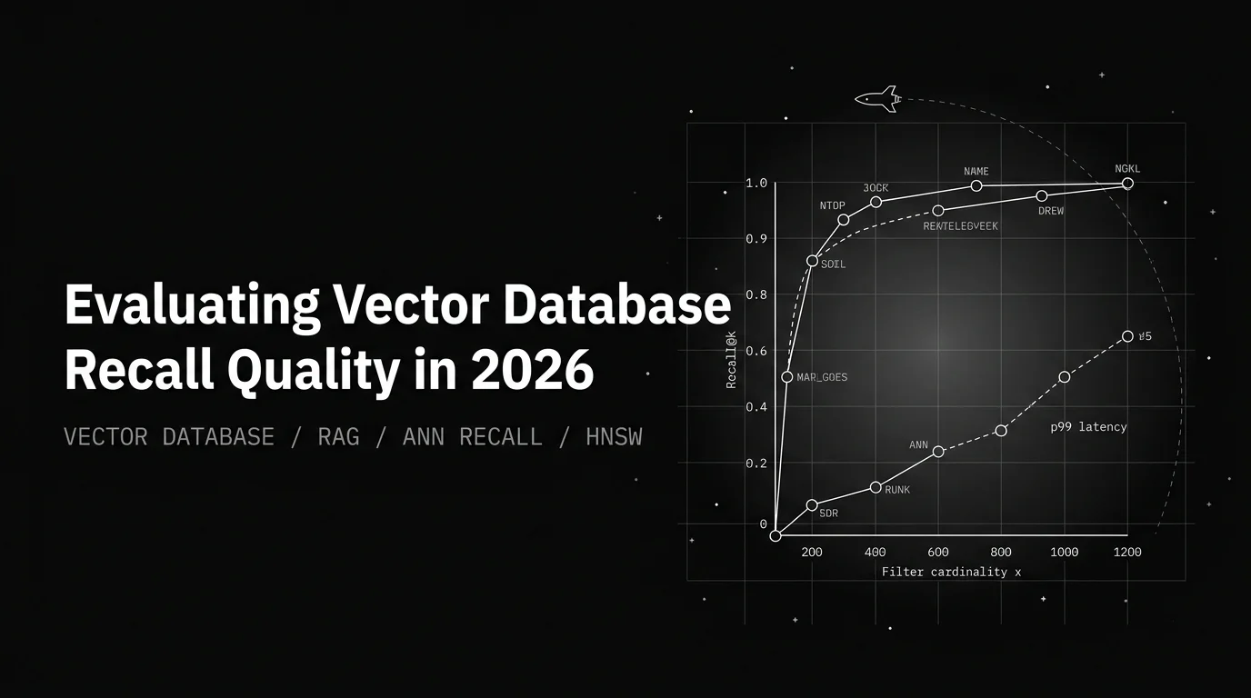
Vendor vector-DB benchmarks are theater. ANN-vs-exact-knn recall on your vectors plus p99 under your filter cardinality is the eval that decides prod.


Vector databases vs knowledge graphs for RAG in 2026. Pinecone, Weaviate, Qdrant, Milvus, Chroma vs Neo4j, GraphRAG, LightRAG. Decision matrix.
