What Is AI Anomaly Detection? Methods, Models, and Where They Fail
A practical breakdown of statistical, distance-based, and deep-learning anomaly detection methods, plus the production failure modes most explainers skip.
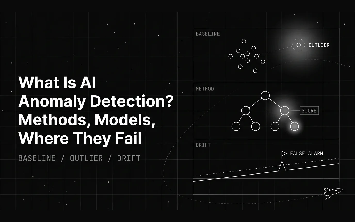
Table of Contents
Anomaly detection shows up everywhere data gets monitored: fraud systems, factory sensors, network traffic, and now AI agent traces. Many beginner-oriented explainers stop at “here are five algorithms,” listed with little context for when each one actually applies in a real system.
Fewer spend comparable space on where each one quietly stops working once it’s running against messy production data. This post covers AI anomaly detection methods and models, then spends equal time on where they fail. A detector that isn’t validated against real incidents is often worse than no detector, because it creates a false sense of coverage nobody checked.
Method descriptions and failure-mode claims below are checked against primary and vendor-neutral sources (linked inline) and current as of August 2026.
TL;DR: AI anomaly detection methods and where they fail
- No single best algorithm. Isolation forest is the common production default for large tabular data with no distributional assumptions; autoencoders handle complex or sequential data at the cost of more compute; one-class SVM fits small, well-separated datasets; ECOD is a newer parameter-free option for non-Gaussian data.
- The failures matter more than the method list. Concept drift, high-dimensional data padded with irrelevant features, imbalanced/unlabeled data, alert fatigue, and anomaly/drift conflation are what quietly break a detector in production — none of them show up in a benchmark comparison.
- Validate against confirmed incidents, not intuition. Track a triage outcome rate (confirmed incidents + new regression checks, divided by total flags) weekly and recalibrate on a schedule instead of treating a threshold as permanent.
What Is AI Anomaly Detection?
AI anomaly detection identifies data points, events, or system behavior that deviate from an expected baseline, using statistical or machine-learning models instead of a fixed manual threshold. Rather than someone hardcoding “alert if latency exceeds 200ms,” a model learns what normal looks like from historical data and flags what doesn’t match it.
Anomalies come in three shapes, following the taxonomy in Chandola, Banerjee and Kumar’s 2009 ACM Computing Surveys review. A point anomaly is a single outlier, like one transaction far larger than a customer’s usual spend. A contextual anomaly is a normal value in the wrong context, like heavy heating use in summer. A collective anomaly is a group of points that’s anomalous together, even though no single point in it looks unusual alone.
The advantage over simple thresholding is adaptability: a learned baseline can shift as the underlying pattern shifts, instead of staying frozen at whatever number someone picked. That same adaptability is also where several of the failure modes covered later come from.
Anomaly detection is often confused with drift monitoring, but they answer different questions. Drift monitoring tracks a population-level shift in data or model behavior over time. Anomaly detection flags individual outliers against a baseline at a single point in time, without necessarily caring how that baseline itself is moving.
They’re related and often deployed together, but conflating them is one of the most common mistakes teams make in practice. A single detector rarely handles both jobs well, and the difference matters more once a system is live, covered in more depth further down.
Where AI Anomaly Detection Is Used
Anomaly detection shows up across a handful of recurring domains. Fraud and transaction monitoring flags spending patterns that don’t match a customer’s history. Network and security teams use it for intrusion detection, watching for traffic that doesn’t match normal usage. Industrial and manufacturing teams apply it to predictive maintenance, catching equipment readings that signal a failure before it happens.
IT and infrastructure teams use it to catch latency spikes and error-rate jumps before they become outages. Increasingly, teams monitoring AI systems apply the same logic to agent traces, LLM outputs, and tool calls, watching for the one execution that quietly went wrong among thousands that looked fine.
The underlying methods (statistical, distance-based, model-based) repeat across all of these domains, so learning one well transfers to the next use case. What changes between them is the features fed into the model: transaction amounts in fraud detection, sensor readings in manufacturing, token-level scores in an LLM pipeline. The next section covers those methods directly, starting with the simplest.
Anomaly Detection Methods
Methods split roughly into three families: statistical, distance or density-based, and model-based approaches, including deep learning. They also split along a second axis of supervised, unsupervised, or semi-supervised, depending on whether labeled anomaly examples exist to train against. Most production anomaly detection ends up unsupervised, because confirmed anomaly labels are rare by definition.
Statistical Methods (Z-score, Moving Averages)
Z-score thresholding flags any point beyond N standard deviations from the mean. Moving averages and exponentially weighted moving averages do the same for time series, comparing each new point against a rolling baseline. Both are cheap, fast, and easy to explain to a non-technical stakeholder.
Both also assume a roughly known distribution, usually Gaussian. They break down on skewed or multi-modal data, where “normal” doesn’t look anything like a bell curve and a single mean and standard deviation stop describing the data well, no matter how the threshold is tuned.
ECOD addresses this specific gap. It estimates a per-dimension empirical cumulative distribution instead of assuming Gaussian shape, making it parameter-free and usable on non-Gaussian data where Z-score thresholding breaks down.
Distance and Density-Based Methods (Clustering, DBSCAN, k-NN)
These methods flag points that sit far from their neighbors or outside a dense cluster. DBSCAN groups points into density-based clusters and treats anything outside them as noise. k-NN distance scoring measures how far a point is from its nearest neighbors and flags large distances.
Both work well on low-dimensional, structured data with clear spatial or categorical grouping. The curse of dimensionality makes distance metrics progressively less meaningful as the number of features grows, since most points start looking roughly equidistant from each other regardless of whether they’re actually anomalous.
That behavior isn’t just intuition. Beyer, Goldstein, Ramakrishnan and Shaft (ICDT 1999) gave the sufficient condition for distance concentration, the point at which nearest-neighbor search stops being meaningful as dimensionality grows.
Durrant and Kabán (2009) later proved the converse: on linear latent-variable data, Euclidean distance does not concentrate as long as the number of relevant dimensions grows no slower than total dimensions. High dimensionality alone is not the problem. Padding with irrelevant features is.
Isolation Forest
Isolation forest randomly partitions the data using recursive splits: it “isolates” observations by randomly selecting a feature, then a split value between that feature’s max and min, and repeating (scikit-learn’s IsolationForest documentation covers the mechanism in detail). Anomalies tend to isolate in fewer splits than normal points because they’re rare and sit apart from the bulk of the data.
It scales well to large datasets and needs no distance metric, which is why it’s a common production default: it makes no assumption about the underlying distribution.
Its main weakness is datasets with varying local density. Isolation forest is sensitive mainly to global outliers; a genuinely anomalous point can sit in a locally dense pocket, isolate slowly, and blend in even though it’s clearly abnormal relative to its immediate neighbors.
Local Outlier Factor, which scores each point against the density of its own neighborhood rather than the dataset as a whole, is the standard fix for exactly this failure mode.
One-Class SVM
One-class SVM learns a boundary around what “normal” data looks like and flags anything that falls outside it, using kernel functions (linear, polynomial, RBF, sigmoid) to handle nonlinear boundaries. On well-separated, moderate-size datasets it can perform strongly.
It gets computationally expensive fast, though: a kernelized one-class SVM’s complexity is at best quadratic in the number of samples, per scikit-learn’s outlier detection guide, which also notes it’s sensitive to outliers in the training set and needs careful nu-hyperparameter tuning to avoid overfitting. Its accuracy degrades further on large, high-dimensional datasets where a clean boundary is harder to define.
Autoencoders and Deep Learning
Autoencoders train a neural network to reconstruct normal data as accurately as possible. Anomalies, being unlike what the network learned, reconstruct poorly, and that reconstruction error becomes the anomaly score. Variants extend the idea: variational autoencoders add a probabilistic layer, and LSTM-based autoencoders handle sequential or time-series data specifically.
These models capture complex nonlinear patterns statistical methods miss entirely, which is why they show up often in high-stakes fraud and security work. That power comes at a cost: they need more data, more compute, and more tuning.
The sharper failure is the opposite of the one people expect. An autoencoder can generalize too well and reconstruct anomalies accurately too, which collapses the reconstruction-error signal the whole method rests on. Gong et al. (ICCV 2019) put it plainly: “sometimes the autoencoder ‘generalizes’ so well that it can also reconstruct anomalies well, leading to the miss detection of anomalies.” Their fix was a memory module that forces reconstruction from stored normal patterns.
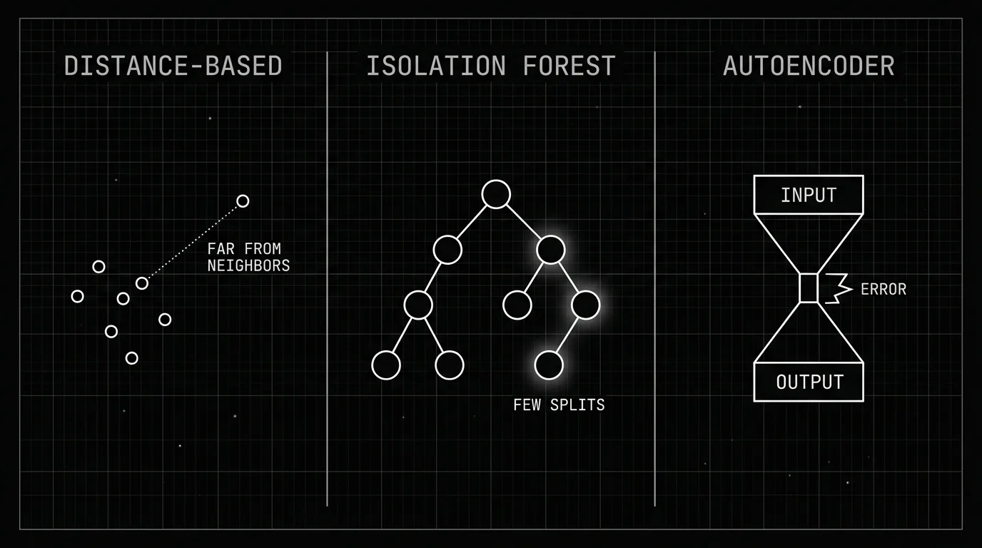
Table 1: Method Comparison
| Technique | How It Works | Best For | Limitations |
|---|---|---|---|
| Z-score / statistical thresholding | Flags points beyond N standard deviations from the mean | Simple univariate metrics, quick baselining | Breaks on non-Gaussian or multi-modal data |
| ECOD | Scores points via per-dimension empirical CDF tail probabilities | Non-Gaussian data, parameter-free baselines | Newer method, less production track record than isolation forest |
| Distance/density-based (DBSCAN, k-NN, LOF) | Flags points far from neighbors, outside dense regions, or locally sparse relative to their own neighborhood | Low-dimensional structured data, spatial clustering, local outliers | Degrades in high dimensions, sensitive to parameter choice, LOF has higher time complexity |
| Isolation Forest | Isolates points via random recursive splits; anomalies split out faster | Large tabular datasets, production default, no distributional assumptions | Weaker on local outliers in datasets with varying local density |
| One-Class SVM | Learns a boundary around normal data using a kernel function | Well-separated, moderate-size datasets | Computationally expensive (up to quadratic in samples), degrades on high-dimensional/large-scale data |
| Autoencoders (incl. VAE/LSTM variants) | Reconstructs input; high reconstruction error flags anomalies | Complex, high-dimensional, or sequential/time-series data | Needs more data and tuning, can generalize well enough to reconstruct anomalies too, less interpretable |
Where AI Anomaly Detection Fails in Practice
The method list above is the easy half. The harder and more useful part is knowing where each one breaks once it’s running against real production data, not a clean benchmark set. That gap is where most anomaly detection deployments quietly stop earning their keep.
Concept Drift and Distribution Shift
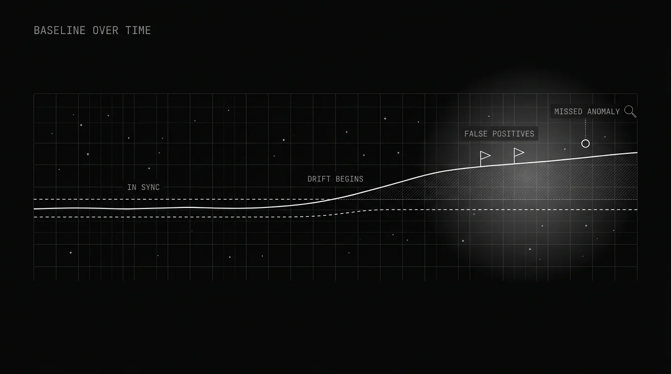
“Normal” changes over time. Seasonal behavior, a product launch, or a new user cohort can all shift the underlying data distribution. Gama et al.’s survey on concept drift adaptation splits that shift into two cases worth keeping apart: real concept drift, a change in p(y|X), the relationship between the inputs and the target; and virtual drift, a change in p(X) alone, with that input-to-target relationship intact.
Unsupervised anomaly detection has no target variable, so the case that breaks it is almost always the second one. A baseline learned from last quarter’s p(X) is being asked to score this quarter’s p(X), and nothing inside the detector knows the two are different.
A static baseline built before that shift either flags legitimate new behavior as anomalous, or quietly re-learns the drifted state as the new normal.
The first outcome is loud: a platform change that shifts typical transaction sizes for new users triggers a spike in false fraud flags until the baseline catches up, and someone opens a ticket about it that week. The second is the dangerous one, because it is silent — the detector absorbs the drifted behavior into its idea of normal and stops flagging the real anomalies now sitting inside it. Nobody files a ticket for alerts that never fired.
High-Dimensional and Sparse Data
As the number of irrelevant features grows, distance-based measures lose their discriminative power: points end up roughly equidistant from each other, so “far from its neighbors” stops meaning much. That is the distance-concentration effect Beyer et al. formalized and Durrant and Kabán bounded, both cited earlier.
The practical read is that dimension count is a proxy, not the cause. A 500-feature dataset where most features carry signal can behave fine; a 50-feature one where 45 are noise will not. Feature selection, dimensionality reduction, or embedding-based approaches are what get distance and density methods working again.
Imbalanced and Unlabeled Data
Anomalies are rare by definition, so there’s rarely enough labeled anomaly data to validate precision and recall with real confidence. The practical consequence is that teams often can’t tell whether they’re missing real anomalies or just annoying people with false alarms, because there’s no ground truth to check either claim against.
Class imbalance also breaks the metric most people reach for first. When positives are a fraction of a percent of the data, ROC-AUC stays flattering because the false-positive rate is divided by a huge negative class, so a detector can look excellent and still bury every real hit under noise. Saito and Rehmsmeier (PLOS ONE, 2015) show the precision-recall plot is the more informative of the two on imbalanced data; report PR-AUC, and quote precision at the recall you actually operate at.
Alert Fatigue and False Positives
A detector tuned too sensitively fires constantly. Teams start ignoring or muting alerts, and the system becomes useless at the exact moment a real anomaly shows up, buried in noise the team has learned to tune out. The fix is threshold calibration against actual confirmed incidents, not an arbitrary sensitivity setting picked once at launch and never revisited.
Anomaly vs. Drift Confusion
Teams often build a single detector and expect it to catch both a lone bad data point and a slow, population-wide shift. Those are different problems that need different detection logic and different response playbooks. A detector tuned for one is often blind to the other, and incidents get missed on whichever side wasn’t the design target.
The drift side has its own taxonomy worth knowing before you build for it — prompt drift, model drift, and eval-score drift are not one phenomenon. What is LLM drift breaks those apart; this post stays on the anomaly side of the line.
Table 2: Failure Mode Comparison
| Failure Mode | Why It Happens | What It Looks Like in Practice |
|---|---|---|
| Concept drift | The definition of “normal” changes over time but the baseline doesn’t update | Sudden spike in false positives after a product change, or real anomalies stop getting flagged |
| High-dimensional / sparse data | Distance and density metrics lose discriminative power as irrelevant dimensions outnumber informative ones | Detector flags almost everything or almost nothing; scores cluster with no clear separation |
| Imbalanced / unlabeled data | Anomalies are rare by definition, little ground truth to validate against | Teams can’t tell if precision/recall is actually good; ROC-AUC looks strong while precision collapses; tuning becomes guesswork |
| Alert fatigue | Detector threshold set too sensitively, without validation against confirmed incidents | On-call teams start ignoring or muting alerts; real anomalies get lost in noise |
| Anomaly/drift conflation | One detector expected to catch both individual outliers and gradual population shift | Detector tuned for one case is blind to the other; incidents get missed on whichever side wasn’t the design target |
How to Choose and Validate an Anomaly Detection Approach
Start with the shape of the problem, not the algorithm. Is the data tabular, sequential, or text and embeddings? How much data exists? Are any confirmed anomaly labels available? Does the use case need real-time scoring or is batch detection fast enough? Those four questions narrow the method list faster than reading another comparison table.
Validation matters more than method choice. Hold out labeled or synthetically injected anomalies to measure precision and recall (and PR-AUC, per the imbalance caveat above) before trusting a detector in production, then recalibrate on a schedule instead of treating a threshold as permanent. A baseline that was accurate at launch drifts out of accuracy the same way the data itself drifts.
One organizational practice most guides skip: track a “triage outcome rate” for every flagged anomaly. Did it become a confirmed incident, a new regression check, or a dismissed alert? That single number tells you whether a detector is earning its alerts or just generating noise someone has to clear every morning.
A worked example: a team reviews 20 anomalies flagged over a week. 3 become confirmed incidents, 5 turn into new regression checks worth keeping, and 12 get dismissed as noise. The triage outcome rate — confirmed incidents plus new regression checks, divided by total flags — is (3 + 5) / 20 = 40%.
The bands we use are a rule of thumb, not a published benchmark: below roughly 20-30%, the alert-fatigue risk described above is usually already setting in and the threshold needs recalibrating; above 60-70%, the detector is often tuned too conservatively and missing real anomalies on the other side. Calibrate the bands against your own incident history rather than adopting ours. Tracking this rate weekly, rather than eyeballing raw alert volume, is what turns “we have a detector” into “we know if the detector is working.”
For AI and LLM systems specifically, the data being monitored is often prompts, responses, tool calls, and traces rather than classic tabular rows. That changes what features feed the detector entirely, and it changes what tooling actually helps, which is where the next section picks up.
How Future AGI Helps Teams Catch Anomalous AI Behavior
As more of the system being monitored is an LLM or agent rather than a fixed pipeline, anomaly detection shifts from tabular features toward traces, prompts, tool calls, and evaluator scores. The tooling underneath that shift looks different from a classic anomaly detection stack, and it’s worth naming concretely rather than staying abstract about it.
Future AGI’s Error Feed scans a sampled slice of an Observe project, decides for itself what failed in each trace, and collapses identical failures into a single issue you work like a ticket, rather than one alert per occurrence. Each issue carries a severity, a status, an assignee, and the fix layer — the part of the system the fix actually belongs in.
Error Feed’s sampling rate is a dial you set, and it starts at zero, so nothing is scanned until you raise it. That is the same cost-versus-coverage tradeoff any production anomaly detector makes, just made explicit instead of buried in a threshold.
Error Feed is the practical equivalent of anomaly detection for agent behavior — the same underlying job as [agent evaluation](https://futureagi, and the production form of that job is covered in evaluating state-graph agent workflows.com/blog/definitive-guide-ai-agent-evaluation-2026/), applied at the individual-trace level instead of the aggregate one. It catches the quietly-wrong trace an aggregate dashboard would average out and never surface on its own.
traceAI, Future AGI’s Apache-2.0, OpenTelemetry-native tracing SDK, ships instrumentors for 50+ LLM, agent, and vector-store frameworks across Python and TypeScript. Those spans are what make this level of visibility possible in the first place. How that tracing layer relates to evaluation and benchmarking as separate but connected disciplines is covered in Future AGI’s breakdown of agent observability vs. evaluation vs. benchmarking.
Protect is the guardrail layer. Each guardrail wraps a check — prompt injection, PII, secrets, content moderation among them — and carries three settings: an action (Block, Warn, Mask, or Log), a stage (pre on the request, post on the response, or both), and a confidence threshold from 0.0 to 1.0.
That’s the security-relevant counterpart to statistical anomaly detection. It’s built for catching abnormal or malicious inputs, not just abnormal data points in a metric, and the threshold dial is the same sensitivity tradeoff the rest of this post describes.
On the evaluation side, Future AGI’s Evaluate layer runs custom evaluation metrics you define for your use case, alongside 70+ built-in templates. A team can score a trace against the exact rubric a generic anomaly score would miss, instead of relying on one fixed statistical signal.
Whether that scoring should run continuously or in scheduled batches is the same tradeoff covered for real-time vs. batch LLM monitoring.
Tracing, evaluation, and guardrails working together mean an anomalous trace isn’t just flagged. It’s routed somewhere a team can actually act on it, which is a gap most classical anomaly detection tooling doesn’t cover for AI systems. Future AGI’s comparison of AI drift detection tools goes deeper into the drift side of this same problem.
Conclusion
AI anomaly detection isn’t one algorithm. It’s a set of methods (statistical, distance-based, isolation forest, one-class SVM, autoencoders) that each make different tradeoffs between speed, interpretability, and how well they handle complex data. Picking one without understanding where it fails is how a detector quietly stops working while still technically running.
Drift, high dimensionality, class imbalance, and alert fatigue are the failure modes that do the most damage, and none of them show up in a benchmark comparison. Validate against real, confirmed incidents rather than intuition, and recalibrate on a schedule instead of assuming a baseline stays true forever.
For teams running LLM or agent systems, the same principles apply to traces and model outputs instead of tabular rows. It’s a fast-growing blind spot worth building for early, before the first missed incident forces the issue, rather than after the damage is already visible to users.
The concrete next step is small: pick one week of flagged anomalies, compute the triage outcome rate on them, and see whether the number justifies the alerts your team is already clearing. If the system you’re monitoring is an agent rather than a pipeline, turn on Error Feed sampling in an Observe project and read the first grouped issue it returns.
Frequently Asked Questions
What is AI anomaly detection?
What is the best algorithm for anomaly detection?
Why does anomaly detection generate so many false positives?
What is the difference between anomaly detection and drift detection?
How do you evaluate an anomaly detection model without labeled data?
AI drift is five different problems wearing one name. We rank the five tools that catch them: Arize, Future AGI, Evidently, WhyLabs, Fiddler.

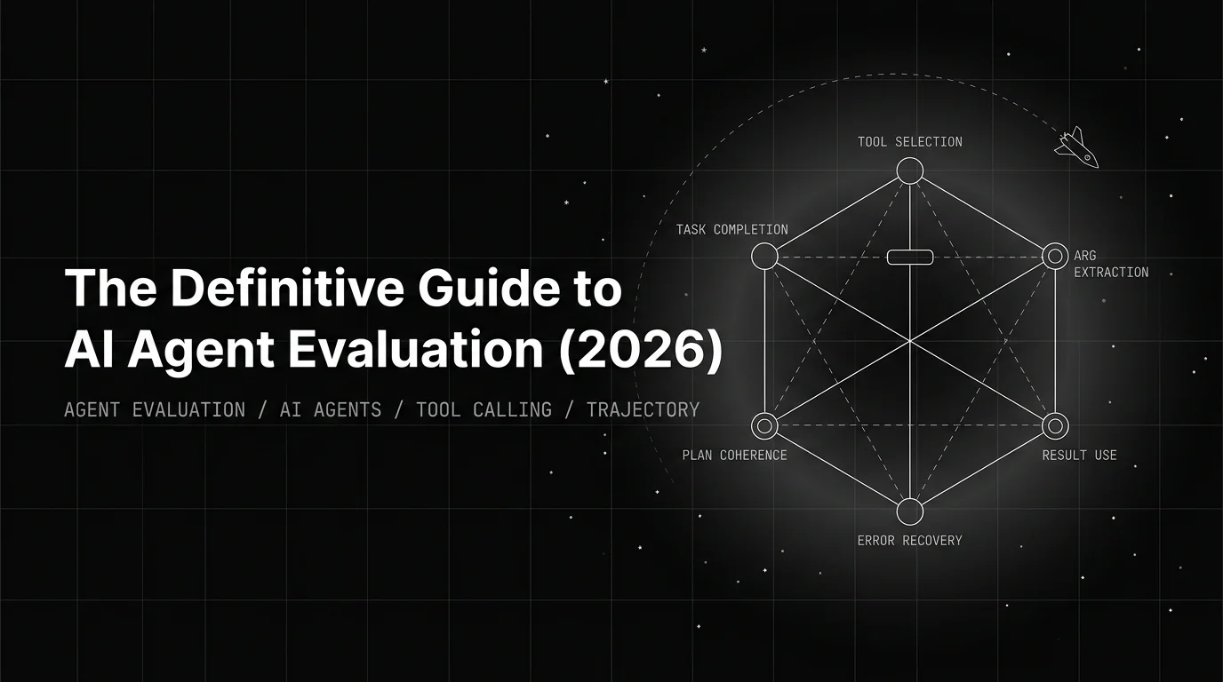
2026 working pattern for AI agent evaluation: six dimensions, six rubrics, a 4-D trajectory score, and a CI gate that beats aggregate scoring.

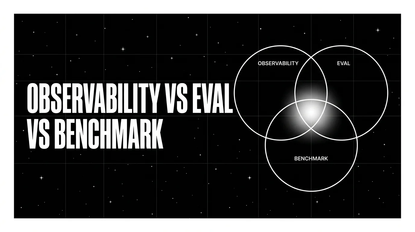
Observability watches. Evaluation judges. Benchmarking ranks. The conceptual map of the three terms agent teams conflate, with metrics, cadence, and tools.