Statistical Significance in LLM Eval Runs
How to calculate statistical significance in an LLM eval run, which test fits pass/fail, category, and score evals, and what your eval set can detect.
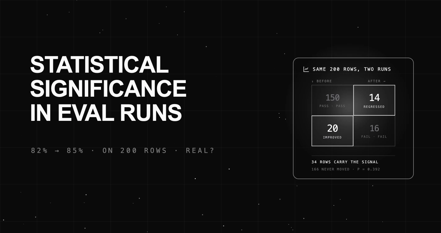
Table of Contents
Evals took over the job A/B tests used to do. Teams no longer ship a prompt change to half their users and wait a week. They run a fixed set of examples through both versions and read the two numbers.
That works right up to the moment the numbers are close. Your eval reads 85% this week against 82% last week, on the same 200 examples, and someone asks whether to ship.
Three points looks like an improvement. Whether it is one depends on something those two numbers do not show: how many of the 200 rows actually changed. The question is not whether the score moved. It is whether an eval set this size can tell the difference.
What Is Statistical Significance in LLM Evaluation?
Statistical significance is a measure of how likely a difference between two eval runs would be if the two versions were actually identical. Teams use it to decide whether a score change justifies shipping. It works by asking how often random chance alone would produce a gap at least this large.
The reason it applies to evals at all is that an eval run is a sample, not a census. Your 200 examples stand in for every input the system will ever see. Score a different 200 and the number moves, even with the model held completely fixed.
Two more sources of movement stack on top of that. If you generate at a temperature above zero, the same input can produce a different output on a different day. If a judge model scores the output, that judge has its own disagreement rate, which a deterministic check does not.
So an eval score is a measurement with error bars, and the aggregate you see on a dashboard does not display them. Significance testing is how you put them back.
Why Do LLM Eval Runs Need Significance Testing?
Because the decisions attached to eval scores are expensive, and the scores move on their own.
Consider a team that ships on any positive delta. When a change makes no real difference and the noise is roughly symmetric, that policy ships noise on about half of the runs that move at all, because a coin-flip movement is positive half the time. Runs that land on exactly the same score pull the real rate somewhat below half.
A team that reverts on every negative delta discards good work at the same rate. Neither can tell, from the aggregate alone, which case it is in.
The problem compounds in a release process. Prompt changes are cheap and frequent, so an eval gate might run dozens of times a month. At that cadence, a gate that fires on unqualified score movement produces a steady stream of false signals, and people learn to ignore it.
There is also a subtler cost. Reporting a 3 point gain that is really noise does not just waste a deploy. It teaches everyone that the eval set is authoritative at a resolution it does not have.
How Do p-Values and Power Relate to Significance?
Two numbers do the work. One tells you how surprising your result is, the other what your eval set could have found in the first place. Most teams look at the first and never the second.
What Is a p-Value?
A p-value is the probability of seeing a difference at least as large as the one you observed, assuming the two versions are actually identical. Low means surprising. The conventional threshold is 0.05.
It is worth being precise about what it does not mean. A p-value of 0.39 is not a 39% chance that the versions are the same. It says that if they were the same, a gap this size would turn up about 39% of the time, which is often enough that you have learned very little.
What Is Statistical Power?
Statistical power is the probability that your test finds a real difference of a given size. The convention is 80%. Power depends on three things: how big the real difference is, how many examples you score, and how much variance each scored row contributes.
For a pass rate that third term is set by the baseline rate itself, since a proportion near 50% carries more variance than one near 95%. For a paired test it is set by something else entirely, which is where the next section turns.
Power is the number that makes eval sets uncomfortable. A small set is not merely less precise. It is close to incapable of detecting the modest, genuine improvements that make up most of the work. An ICLR 2025 blogpost on rigour in language model evaluations argues published benchmarks have the same problem.
This post is about reading a run you already have. Turning power into a target sample size before you run anything, including the minimum detectable effect and the arithmetic that follows from it, belongs to our A/B testing playbook for LLM prompts and is not repeated here.
What Is the Formula for Significance in an Eval Run?
When both runs score the same examples, the right comparison is not the two totals. It is the rows where the two runs disagreed.
Take a real shape. A pass or fail eval, 200 rows, scored before and after a prompt change.
| After: pass | After: fail | |
|---|---|---|
| Before: pass | 150 | 14 |
| Before: fail | 20 | 16 |
Baseline is 164 of 200, or 82%. The new version is 170 of 200, or 85%. The net gain of 6 rows is the difference between 20 rows that started failing and now pass, and 14 that went the other way.
The 150 rows both runs passed and the 16 both runs failed tell you nothing about which version is better. Both versions handled them identically. Only the 34 disagreements carry information, which is what McNemar’s test uses:
McNemar's exact test, on the 34 disagreements:
  p = 2 x P(X >= 20), where X ~ Binomial(34, 0.5)

  the two-sided probability of a split at least this lopsided,
  if improvement and regression were equally likely
Running that on these counts gives p = 0.392. If the two prompt versions were truly identical, you would see a split at least this lopsided about 39% of the time. That is not evidence of an improvement.
Note what the aggregate hid. It reported “82% to 85%” across 200 rows, when 166 of those rows never moved at all and the entire result rests on 34.
This is not a niche preference. Evan Miller’s Adding Error Bars to Evals (Anthropic, November 2024) makes it one of five recommendations: when comparing two models, conduct “statistical inference on the question-level paired differences, rather than the population-level summary statistics”.
The row is the unit of analysis. The dashboard number is not.
Which Eval Types Need Which Test?
An eval run returns one of three things: pass or fail, a number, or a category. The shape of that output decides the test, and using the wrong one either wastes data or invents confidence you do not have.
If you are still choosing what to measure, start from the eval metrics themselves and come back here.
| Your eval returns | Same rows in both runs | Use | Why |
|---|---|---|---|
| Pass or fail | Yes | McNemar’s test | Only rows that changed carry information |
| Pass or fail | No | Two proportion z test | Unpaired, so every row’s difficulty becomes noise |
| A category | Yes | Stuart-Maxwell test on the transition matrix | The paired form of the same question, and it reduces to McNemar at two categories |
| A category | No | Chi-square, or Fisher exact for small counts | Compares two independent distributions |
| A number or score | Yes | Paired t test, or a paired bootstrap interval | Pairing removes example difficulty as a variable |
Pass or Fail Evals
This is the common case, and the worked example above is it. Use McNemar when the runs are paired, which they are whenever you re-run a fixed eval set.
If the two runs scored different examples, McNemar does not apply and you need a two proportion z test. On the same totals as above, that test returns p = 0.419 rather than 0.392. Pairing is doing real work even when both verdicts agree, and on closer results that gap is what decides the call.
Category Evals
When an eval grades into three or more buckets, collapsing to pass or fail throws away where the movement happened. Here are two runs over the same 200 rows, reported the way a dashboard reports them:
| Outcome | Before | After |
|---|---|---|
| Correct | 120 | 132 |
| Partially correct | 40 | 38 |
| Wrong | 40 | 30 |
The temptation is to run a chi-square test on that table. Do not. Chi-square compares two independent distributions, and these are the same 200 rows scored twice. It is the same mistake as comparing the two totals in the pass or fail case.
Bucket totals also cannot tell you where anything went. Twelve more rows are correct, but you cannot see whether twelve wrong answers became correct or forty rows churned in both directions. Only the transition matrix shows that, and it is the 2x2 table from earlier with more buckets:
| After: correct | After: partial | After: wrong | |
|---|---|---|---|
| Before: correct | 104 | 10 | 6 |
| Before: partial | 16 | 22 | 2 |
| Before: wrong | 12 | 6 | 22 |
Its marginals are identical to the table above, so a dashboard shows the same picture either way. What it adds is that 52 of the 200 rows changed category, in both directions: 34 moved up the scale and 18 moved down.
Twelve is smaller than both of those numbers. One reason is that a row moving from wrong to partially correct is a real improvement that never reaches the bucket the headline counts.
The paired test for this shape is the Stuart-Maxwell test, which asks whether the two distributions differ once pairing is accounted for, and which reduces to McNemar at two categories. On this matrix it gives chi-square = 4.663 on 2 degrees of freedom, p = 0.097.
One detail to expect if you check that reduction yourself. At two categories Stuart-Maxwell reduces to the McNemar chi-square without continuity correction, not to the exact binomial used earlier. On the 2x2 above it returns p = 0.303 rather than 0.392. Both are McNemar; they are the asymptotic and exact forms of it.
The naive chi-square returns p = 0.359 on the same data. Neither clears 0.05, but they are not the same answer, and on a result nearer the threshold that gap decides the call.
Two cautions. The asymptotic Stuart-Maxwell statistic is approximate when off-diagonal cells are small, and the smallest here is 2, so treat p = 0.097 as indicative rather than exact. An exact or permutation version is safer at these counts.
Second, if you intend to ask a directional question instead, such as whether more rows improved than regressed on an ordered scale, choose that test before you look at the matrix. The same 52 rows support several different questions, and picking the one that reads best afterwards is how teams talk themselves into shipping noise.
Judge Score Evals
When your eval returns a continuous score rather than a verdict, the paired t test is the standard choice for roughly symmetric paired differences.
Wilcoxon signed-rank is often named as the fallback for skewed deltas, but it is not a general substitute. It carries its own assumptions and discards tied rows, which are common when a judge scores on a coarse scale. For bounded or spiky judge scores, a paired bootstrap interval on the per-row delta is usually more defensible.
Designing that comparison in advance is a different job from reading a run you already have. Choosing the effect size you want to detect, sizing the set for it, and handling judge disagreement are covered separately.
When Should You Not Run a Significance Test?
Significance is the wrong tool more often than statistics posts admit.
Skip it when the difference is obvious. A change that takes a pass rate from 60% to 85% on a fixed set does not need a test to be believed, and running one adds ceremony without adding information.
Skip it when the result is not the decision. If a change is required for compliance or fixes a specific reported failure, a p-value has no vote. Ship it and use the eval to check you did not break something else.
Be careful when the eval set is not representative. Significance tells you a difference is unlikely to be noise on the examples you scored. It says nothing about whether those examples resemble production traffic. A significant result on an unrepresentative set is a confident answer to the wrong question.
And treat significance and importance as separate. A large enough eval set can make a 0.4 point gain significant. Whether 0.4 points is worth a deploy is a product judgment that no test will make for you.
How Do You Run These Tests in Python?
For a paired pass or fail eval, McNemar’s exact test is a two-sided binomial test on the disagreements, which means scipy.stats.binomtest alone is enough. Export the per-row results of both runs, count the two disagreement types, and test:
from scipy.stats import binomtest

# both runs scored the same 200 rows
regressed = 14   # passed before, fails now
improved  = 20   # failed before, passes now

discordant = improved + regressed
result = binomtest(improved, n=discordant, p=0.5)

print(f"rows that changed: {discordant} of 200")
print(f"p = {result.pvalue:.3f}")
# rows that changed: 34 of 200
# p = 0.392
For a category eval, build the transition matrix from the same export and hand it to statsmodels, which implements Stuart-Maxwell as the homogeneity test on a square paired table:
import numpy as np
from statsmodels.stats.contingency_tables import SquareTable

# rows = category before, columns = category after, same 200 rows
#                        correct  partial  wrong
transitions = np.array([[   104,     10,     6 ],   # was correct
                        [    16,     22,     2 ],   # was partially correct
                        [    12,      6,    22 ]])  # was wrong

result = SquareTable(transitions).homogeneity()
moved = transitions.sum() - np.trace(transitions)

print(f"rows that changed category: {moved} of {transitions.sum()}")
print(f"chi2 = {result.statistic:.3f}, dof = {result.df}, p = {result.pvalue:.3f}")
# rows that changed category: 52 of 200
# chi2 = 4.663, dof = 2, p = 0.097
Note that this needs the transition matrix, not two rows of bucket totals. If your export only carries the per-run counts, the paired test is not available to you and you are back to the unpaired chi-square, which is the weaker question.
As a build gate, compare the p-value to a threshold you set in advance and fail the build only on a significant regression. Treat an inconclusive result as inconclusive rather than as a pass, and log it, so a gate that never fires becomes visible.
One caveat grows with cadence. A two-sided gate at the conventional 5% threshold is, by construction, wrong about 5% of the time when nothing has changed. About half of those errors point the wrong way, so a gate that fails only on regressions fires falsely about 2.5% of the time.
Run it on every pull request and that becomes a steady trickle of false regressions, which is the alert fatigue this article opened with.
If your gate runs often, set a stricter threshold, act only on repeated signals rather than single runs, or use a sequential test built to be checked repeatedly. Correcting for repeated testing is covered in our prompt A/B testing playbook.
How Do You Monitor Eval Significance in Production?
Every test above needs the same input: per-row results from two runs over the same examples. Aggregates cannot be un-averaged, so if your tooling only stores a mean, none of this is available afterwards.
Future AGI’s experiments run every prompt and model configuration against the same dataset and score them with the same evals, which makes pairing structural rather than something you arrange by hand.
The Experiments product page puts the useful part plainly: “Create a base column with your current prompt output, then run new prompt variants against the same dataset. See exactly which rows improved, which regressed, and by how much.”
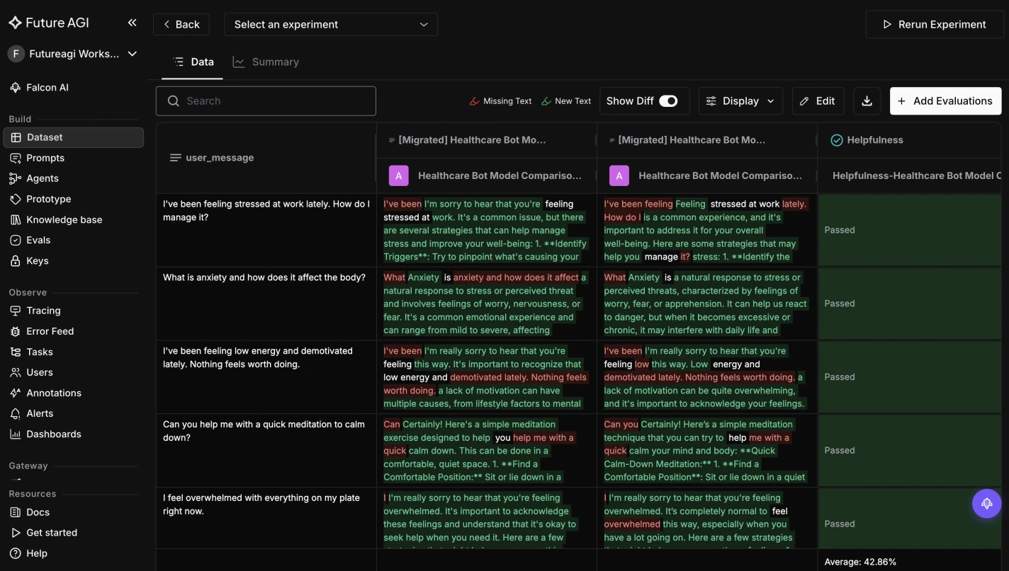
What that view keeps is the per-row verdict for each configuration, side by side. Counts of rows that improved and rows that regressed fall straight out of it, and those are exactly the two numbers McNemar’s test consumes.
The same holds on the evaluation side. Every run “produces a result for each row, span, or test input it scores”, and aggregates roll up on top of those results rather than replacing them.
Where the API exposes a per-span rollup, it returns the raw per-row eval result with no averaging applied beside it.
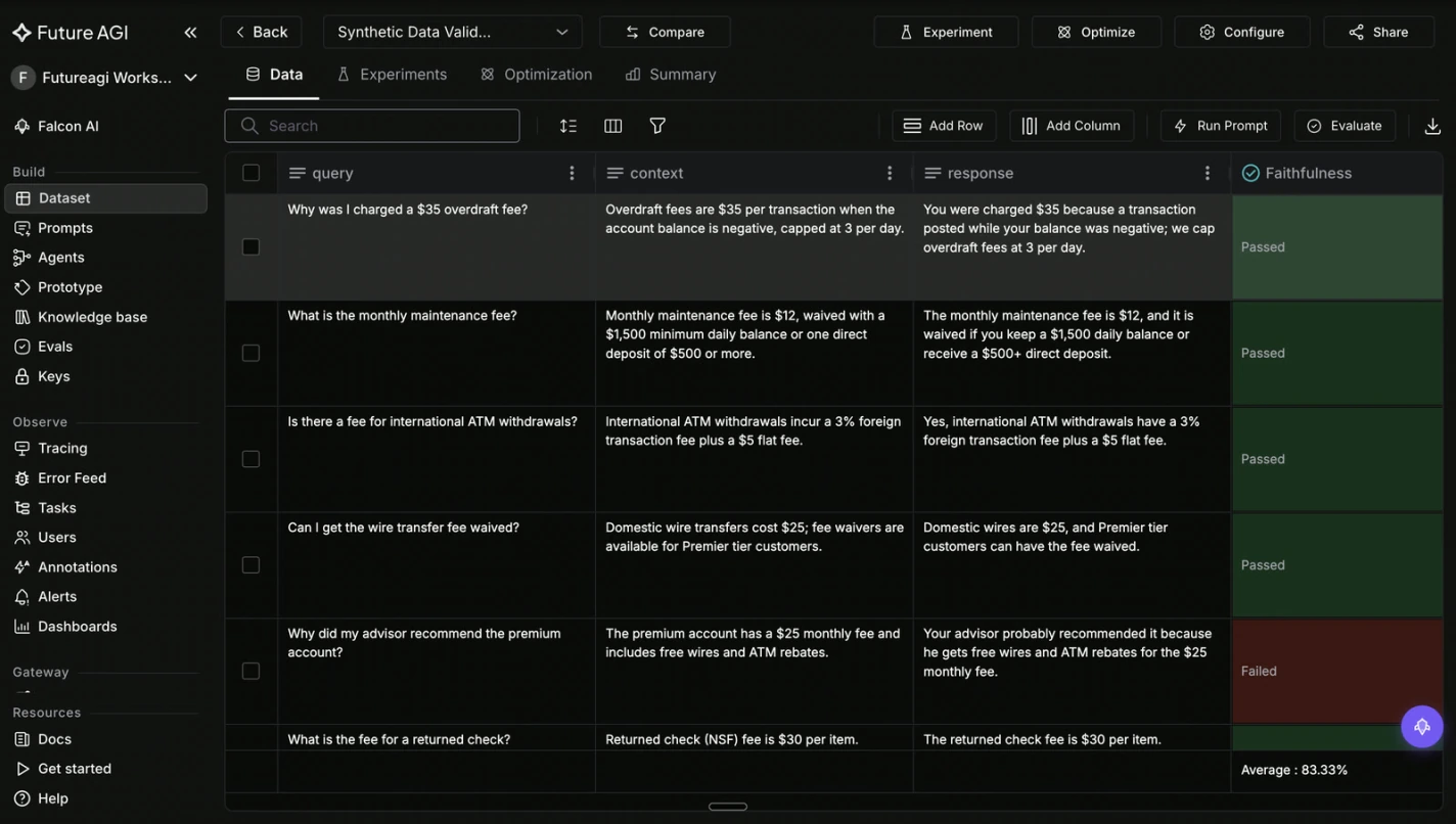
The 83.33% average above is the number a dashboard reports. The Pass and Fail column beside it is the number a significance test needs.
One more thing has to stay fixed between runs. Edit an eval’s criteria or threshold and the two runs no longer measure the same thing, which makes any test comparing them meaningless.
Eval templates are versioned for that reason: each version is “a frozen copy of the exact criteria and threshold, so you can pin a run to a specific version”.
Which Eval Differences Are Worth Acting On?
Work out what your eval set can resolve, then only act on differences above that line. At a baseline pass rate near 80%, with a two-sided 5% threshold and 80% power, an unpaired comparison of two independent samples resolves this much:
| Rows scored in each run | Smallest gain an unpaired test can detect |
|---|---|
| 200 rows | about 10 points |
| 500 rows | about 6.6 points |
| 2,000 rows | about 3.4 points |
Read that column as rows per run, not rows in total. Split 200 rows into two arms of 100 and the same test resolves about 13 points, not 10.
Pairing changes that arithmetic rather than simply improving it. Under McNemar the binding quantity is not the baseline pass rate but the share of rows that disagree between the two runs.
At 200 rows, an eval where 17% of rows change resolves about 8 points, better than the unpaired figure. One where 30% change resolves about 11, slightly worse. Pairing helps when your two versions agree on most rows, which is the usual case for a prompt edit, but estimate that rate from a pilot run rather than assuming it.
So pair your runs, then size them against the disagreement rate you actually observe. Keep category outcomes as a transition matrix instead of collapsing them, because the collapse discards both the detail that explains the change and the pairing that gives the test its power.
And when a result comes back inconclusive, read it as inconclusive. It means this eval set cannot see a difference this small, which is a fact about your measurement rather than a verdict on your change.
Frequently Asked Questions About Statistical Significance in LLM Evals
What Counts as a Statistically Significant Difference Between Two Eval Runs?
The usual bar is a p-value below 0.05, meaning a gap this large would appear less than 5% of the time if the two versions were identical. That threshold is a convention, not a law.
What matters more is that you fix the threshold before you look at the result, and that you pair the runs so the same examples are scored twice. An unpaired comparison on the same totals typically looks weaker, because it treats every row’s difficulty as noise.
Which Statistical Test Should I Use for a Pass or Fail Eval?
Use McNemar’s test when both runs scored the same examples, which is the normal case for an eval set. It looks only at the rows where the two runs disagreed, because rows that both runs passed or both failed carry no information about which version is better.
If the two runs scored different examples, use a two proportion z test instead, and expect to need considerably more data for the same confidence. For evals that grade into three or more categories, the paired equivalent is the Stuart-Maxwell test, which reduces to McNemar when there are only two.
Is 200 Examples Enough for an LLM Eval Set?
It depends on the improvement you want to detect and on how many rows change between runs. Unpaired, at an 80% baseline with a 5% threshold and 80% power, 200 examples in each run resolve about 10 percentage points, 500 resolve about 6.6 and 2,000 resolve about 3.4.
Pairing changes this: under McNemar the binding quantity is the share of rows that disagree, so 200 rows resolve about 8 points at 17% disagreement and about 11 at 30%. Estimate that rate from a pilot run.
Why Did My Eval Score Move If Nothing Is Really Different?
Because an eval run samples. Each run scores a finite set of examples, and if the model is sampling at a non zero temperature or a judge model is scoring the output, the same input can produce a different result on a different day.
Small movements in an aggregate score are the expected behaviour of a noisy measurement, not evidence that anything changed.
What Should I Do When a Significance Test Comes Back Inconclusive?
An inconclusive result means your eval set cannot resolve a difference this small, not that the versions are identical. Pair the runs if you have not already, keep category outcomes instead of collapsing them to pass or fail, and look at which specific rows changed rather than the aggregate.
If the change still matters, the honest options are to grow the eval set or to only ship differences large enough for your current set to detect.
Sources
- Evan Miller, Adding Error Bars to Evals: A Statistical Approach to Language Model Evaluations, Anthropic, November 2024.
- Towards more rigorous evaluations of language models, ICLR Blogposts 2025.
scipy.stats.binomtestandstatsmodelsSquareTable.homogeneity, the implementations used for every p-value in this article.
Every figure in this post was computed rather than cited, as of 2026-07-31. The p-values are reproducible from the code above.
The detectable-gain tables are not. They come from a normal-approximation power calculation at a two-sided alpha of 0.05 and 80% power: the standard two-sample formula for the unpaired figures, and the discordant-pair formula for the McNemar figures, in which the binding quantity is the disagreement rate rather than the baseline pass rate.
Different normal approximations of the paired formula disagree by roughly a tenth of a point, so treat these as the scale of what a set can resolve rather than as exact thresholds.
Frequently Asked Questions
What counts as a statistically significant difference between two eval runs?
Which statistical test should I use for a pass or fail eval?
Is 200 examples enough for an LLM eval set?
Why did my eval score move if nothing is really different?
What should I do when a significance test comes back inconclusive?

A/B testing LLM prompts without power analysis is theater. The 2026 playbook: MDE, sample sizing, matched pairs, bootstrap CIs, bandits, and rollout.


There aren't 50 LLM eval metrics. Three primitive families and eight rubrics matter in production. 2026 reference with CI gate and per-trace eval cascade.


Deterministic vs LLM-judge isn't a pick. It's a cascade. Where each wins, where each breaks, and the layering that drops eval cost 95% in production.