Mean Squared Error (MSE) in Machine Learning: Formula, RMSE, MAE, and R-Squared
Complete MSE guide for 2026. Formula, Python example, when MSE beats MAE or RMSE, R-squared comparison, outlier sensitivity, neural network loss use cases.
Table of Contents
Mean Squared Error (MSE) in Machine Learning: Formula, RMSE, MAE, and R-Squared
MSE stands for Mean Squared Error. It is a regression metric equal to the average of the squared differences between a model’s predicted values and the actual values, written as MSE = (1/n) Σ (yᵢ − ŷᵢ)². Lower is better, zero means every prediction was exact, and the result carries the squared units of whatever you are predicting.
That is the whole definition. The rest of this guide covers why the squaring step matters, when MSE misleads you, and what to use instead when it does.
MSE is both an evaluation metric and a training loss: it is the function gradient descent minimizes when you train a regression network. This guide covers the MSE formula, a working Python example, when to prefer MSE over MAE or RMSE, the relationship to R-squared, and how MSE behaves in neural networks and ensemble methods.
TL;DR: MSE, RMSE, MAE, and R-Squared at a Glance
| Metric | Formula | Units | Outlier sensitivity | When to use |
|---|---|---|---|---|
| MSE | mean of (y - y_hat) squared | Target units squared | High | Default regression loss, gradient descent |
| RMSE | square root of MSE | Target units | High | Reporting error in original units |
| MAE | mean of absolute (y - y_hat) | Target units | Low | Outlier-robust regression error |
| R-squared | 1 minus MSE divided by the population variance of the target | Unitless (1 perfect, 0 mean predictor, negative is worse) | Indirect | Communicating fit quality across teams |
| Huber loss | Quadratic for small errors, linear for large | Mixed scale (delta-dependent) | Medium | Mix of MSE smoothness and MAE robustness |
Mean Squared Error Formula
The mean squared error formula is:
MSE = (1 / n) × Σⁿᵢ₌₁ (yᵢ − ŷᵢ)²
Where:
- yᵢ is the actual value from the dataset
- ŷᵢ is the predicted value from the model
- n is the number of observations
- Σ sums the squared error across all n observations
The squaring step ensures both over-predictions and under-predictions contribute positively, and it weights larger deviations more heavily than smaller ones. The result is non-negative, has the units of the target variable squared, and equals zero only when every prediction is exactly correct.
Worked example
Suppose a model predicts house prices for four houses, in thousands of dollars:
| Actual (y) | Predicted (ŷ) | Error (y − ŷ) | Squared error |
|---|---|---|---|
| 200 | 210 | −10 | 100 |
| 350 | 340 | 10 | 100 |
| 275 | 295 | −20 | 400 |
| 410 | 400 | 10 | 100 |
Sum of squared errors = 100 + 100 + 400 + 100 = 700. Divide by n = 4, and MSE = 175.
Two things to notice. First, the units are thousands-of-dollars squared, which is not a quantity anyone can reason about directly, so you would report RMSE = √175 ≈ 13.2 thousand dollars instead. Second, the single 20-unit error contributed 400 of the 700 total, more than the other three errors combined. That is the squaring step doing exactly what it is designed to do, and it is also the reason a single bad outlier can dominate the score.
What Is Mean Squared Error
Conceptually, MSE answers one question: on average, how far off is this model, with big misses counting for disproportionately more than small ones?
It is worth being precise about why the errors get squared, because two other things would also work. Taking the raw average of (y − ŷ) fails immediately: over-predictions and under-predictions cancel, so a model that is wildly wrong in both directions can score zero. Taking absolute values fixes the cancellation and gives you MAE, which is a perfectly good metric. Squaring does something MAE does not: it makes the error surface smooth and differentiable everywhere, which is what lets gradient descent optimize it directly, and it encodes a specific opinion that one 10-unit error is worse than ten 1-unit errors.
That opinion is a modelling choice, not a mathematical fact. When it matches reality, MSE is the right metric. When your large errors are measurement noise rather than genuine model failure, it is the wrong one, and the sections below cover what to use instead.
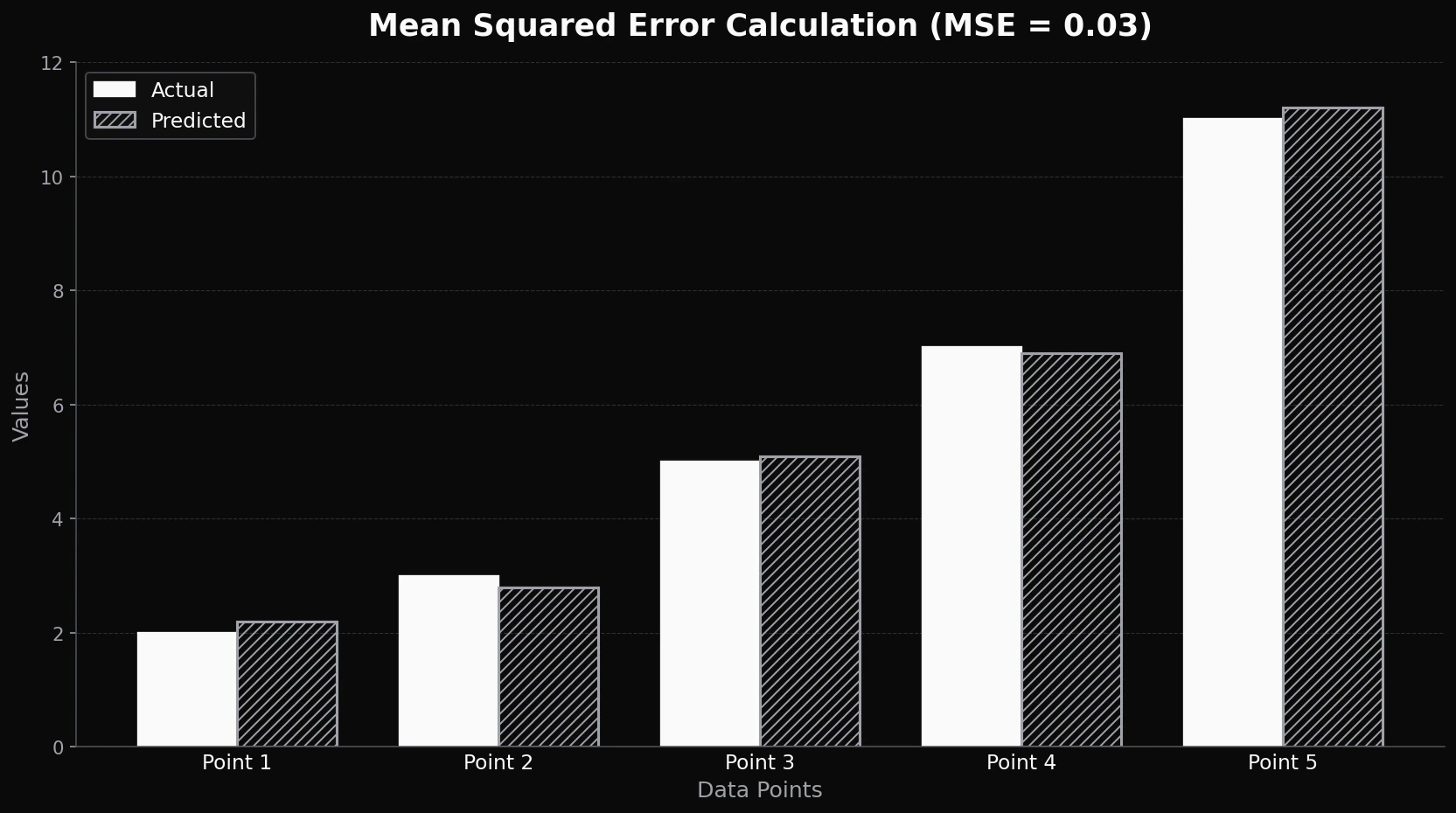
Figure 1: Mean Squared Error Calculation showing Actual vs Predicted values across five data points
How MSE Differs from MAE and RMSE
MAE (Mean Absolute Error) takes the absolute value of each error instead of squaring it. That keeps the metric in the original units and treats all errors linearly, so a single 10-unit error contributes the same as ten 1-unit errors. MAE is therefore more robust to outliers but harder to optimize with gradient methods because it is not differentiable at zero.
RMSE (Root Mean Squared Error) is the square root of MSE. It rescales MSE back into the original units of the target, which makes it easier to communicate. RMSE and MSE rank models identically (lower MSE always means lower RMSE), so they are interchangeable for model selection.
RMSE vs MSE: Which Should You Report?
Short answer: optimize MSE, report RMSE.
They contain identical information. RMSE is defined as √MSE, and because the square root is monotonic, any model that beats another on MSE also beats it on RMSE. There is no scenario where the two disagree about which model is better. The choice between them is entirely about what a number means to whoever reads it.
| MSE | RMSE | |
|---|---|---|
| Units | Target units, squared | Target units |
| Interpretable to a stakeholder | No | Yes |
| Use as a training loss | Yes, standard | Rarely, adds a needless square root |
| Ranks models | Identically to RMSE | Identically to MSE |
| Outlier sensitivity | High | High, but compressed by the root |
In the worked example above, MSE = 175 “thousand-dollars squared”, which means nothing to anyone. RMSE ≈ 13.2 thousand dollars means the model is typically off by about thirteen thousand dollars, which a product manager can act on.
Two details people get wrong. First, RMSE is not the average error, and it is not MAE. Because of the squaring inside, RMSE is always greater than or equal to MAE, and the gap between them widens as your errors become more uneven. Comparing RMSE against MAE is actually a quick diagnostic: if RMSE is far above MAE, your error is concentrated in a few large misses rather than spread evenly. Second, taking the root does not make RMSE robust to outliers. It compresses the scale but the squaring already happened, so a single dominant outlier still drives the number.
For training, stick with MSE. The extra square root adds computation and changes the gradient scale without changing which minimum you reach.
MSE as a Loss Function: PyTorch and TensorFlow
Every major framework ships MSE as a built-in regression loss, because it is the default choice for continuous-target networks.
import torch
import torch.nn as nn

criterion = nn.MSELoss()          # reduction="mean" by default
predictions = torch.tensor([210.0, 340.0, 295.0, 400.0])
targets     = torch.tensor([200.0, 350.0, 275.0, 410.0])

loss = criterion(predictions, targets)
print(loss.item())                # 175.0, matching the worked example above
import tensorflow as tf
mse = tf.keras.losses.MeanSquaredError()
print(mse([200.0, 350.0, 275.0, 410.0], [210.0, 340.0, 295.0, 400.0]).numpy()) # 175.0
# Or as a compile-time argument
model.compile(optimizer="adam", loss="mse", metrics=["mae"])Three things worth knowing when you use it as a loss rather than a report metric:
- The
reductionargument matters. PyTorch’snn.MSELossdefaults toreduction="mean", which averages over every element. Switching toreduction="sum"makes your effective learning rate scale with batch size, which is a common source of training instability that looks like a bad learning rate. - Scale your targets. MSE gradients are proportional to the error magnitude, so an unscaled target in the tens of thousands produces enormous initial gradients. Standardize or normalize the target and the same architecture usually trains without exploding.
- Use Huber when the data is dirty.
nn.HuberLossandtf.keras.losses.Huberbehave quadratically for small errors and linearly for large ones, which keeps MSE’s smooth gradients near the optimum while capping the influence of outliers.
Why MSE Matters in Machine Learning
Measuring Regression Model Accuracy
MSE provides a single, quantitative number that summarises how close predictions are to truth. Lower MSE means predictions are tighter around the actual values. Higher MSE means the model is off, sometimes systematically and sometimes only on a few high-leverage points.
Classic use cases include:
- Stock price prediction. MSE measures how far model output is from realized prices. Squaring penalises blowups more than chronic small drift, which matters when a single bad day can wipe out a quarter.
- Sales forecasting. A retailer evaluates monthly forecasts with MSE to flag regions and seasons where prediction error is concentrated.
- Weather prediction. Meteorologists track MSE of temperature and rainfall forecasts to decide when a model is good enough to release publicly.
Why Gradient Descent Likes MSE
The training loop computes MSE on a mini-batch, takes the gradient with respect to model parameters, and updates the parameters with an optimizer like Adam or SGD. See the framework code above for the PyTorch and TensorFlow calls.
Three properties make MSE well behaved for gradient descent:
- Smoothness. The squared-error surface is differentiable everywhere, which keeps the gradient stable.
- Convexity in linear models. For linear regression, the MSE surface is globally convex, so gradient descent converges to the unique optimum.
- Strong penalty on outliers. The squared term keeps the model focused on large errors during training. This is helpful when large errors are costly and unhelpful when they are noise.
Insights MSE Provides About Model Performance
MSE alone tells you the average squared error. Pairing MSE with residual analysis reveals where the model struggles:
- A handful of large residuals dragging up MSE usually points to outliers, leverage points, or missing features for a sub-population.
- A flat residual plot with high MSE points to underfitting.
- A residual plot that fans out with increasing predictions points to heteroscedasticity. One global MSE hides range-dependent error patterns in that case, so segmented metrics or residual plots are required to diagnose where the model is failing.
How to Calculate MSE: Step-By-Step
To compute MSE by hand:
- Subtract the predicted value from the actual value for each observation.
- Square each difference.
- Sum the squared differences.
- Divide by the number of observations.
Example:
- Actual values: [5, 7, 9]
- Predicted values: [6, 6, 10]
- Errors: [-1, 1, -1]
- Squared errors: [1, 1, 1]
- MSE: (1 + 1 + 1) / 3 = 1.0
Working Python Example with NumPy and Scikit-Learn
import numpy as np
from sklearn.metrics import mean_squared_error

y_actual = np.array([5, 7, 9])
y_predicted = np.array([6, 6, 10])

# Manual calculation
mse_manual = np.mean((y_actual - y_predicted) ** 2)

# Scikit-learn equivalent
mse_sklearn = mean_squared_error(y_actual, y_predicted)

rmse = np.sqrt(mse_sklearn)
print(f"MSE: {mse_manual:.4f}")
print(f"MSE (sklearn): {mse_sklearn:.4f}")
print(f"RMSE: {rmse:.4f}")
mean_squared_error is the standard reference implementation. Use it for production code rather than rolling your own to avoid edge-case bugs with empty arrays or NaN handling.
Common Pitfalls in MSE Calculation
- Outliers. A single 100-unit error contributes 10,000 to the sum of squares, which dwarfs ninety-nine 1-unit errors that total only 99. Inspect residuals before trusting MSE.
- Scale dependency. MSE is in the squared units of the target. Comparing MSE across models that predict different targets is meaningless without normalization.
- Train versus test split. Always report MSE on a held-out test set, not the training set, to detect overfitting.
What Is a Good MSE Value?
There is no universal threshold, and any source that gives you one is wrong.
The reason is in the units. MSE is measured in the squared units of your target variable, so its magnitude depends entirely on what you are predicting. An MSE of 175 is excellent when predicting house prices in thousands of dollars and catastrophic when predicting a probability between 0 and 1. The number is not comparable across datasets, across target scales, or even across the same dataset after you change the units.
What makes an MSE good or bad is always a comparison. Three that actually work:
- Against the mean baseline. Compute the MSE of a model that ignores every feature and always predicts the training mean. Your model must beat it, and by a margin worth the complexity. This comparison is exactly what R-squared formalises: R² = 1 − (MSE / variance of the target), where that variance is the population form dividing by n, matching MSE’s own denominator. R² = 0 means you tied the mean predictor and negative R² means you lost to it.
- Against the previous model. For an existing production system, the only MSE that matters is the incumbent’s on the same held-out set. A 5 percent reduction that holds up on test data is a real result.
- Against the cost of being wrong. Convert to RMSE, put it in target units, and ask whether an error of that size is acceptable to the business. If your demand forecast has an RMSE of 400 units and the warehouse holds 300, the model is not usable regardless of how the number compares to anything else.
The one absolute statement worth making: an MSE of exactly zero on training data is not a good result, it is a warning. It almost always means the model has memorised the training set or a feature is leaking the target.
How to Interpret MSE Results
High MSE
A high MSE indicates large prediction errors on average. Common causes:
- Underfitting (model is too simple for the relationship)
- Inadequate feature engineering or missing predictors
- Data quality issues like mislabeled targets, missing values, or measurement noise
Low MSE
A low MSE indicates predictions are close to actual values. Always confirm the score on test data; a very low training MSE can hide overfitting. Cross-validation and a held-out test set give a more honest read.
Balancing MSE with RMSE and R-Squared
R-squared rescales error into a unitless fit score where 1 is perfect, 0 matches the mean predictor, and negative values mean the model is worse than the mean baseline. R-squared = 1 minus (MSE / variance of target). For a clear walkthrough see R-squared model accuracy. RMSE rescales MSE back into the target units. Most reports include all three, plus a residual plot for diagnostics.
Practical Applications of MSE
Forecasting and Time Series
Time-series models use MSE to track forecast error against realized values. A retail chain that forecasts monthly sales by region uses MSE to flag regions where forecast error has grown, often a signal of missing seasonal or regional features. For drift over time see model vs data drift.
Pricing and Recommendation Models
E-commerce platforms use MSE to evaluate predicted optimal prices against actual customer behavior. Recommendation engines that predict ratings (Netflix-style 1-to-5 stars before they switched to thumbs) use MSE on the predicted rating vector against held-out ratings.
Computer Vision Regression Tasks
CNNs that regress bounding-box coordinates or pixel values use MSE on the coordinate vector. Object-detection losses like the Smooth L1 loss in Fast R-CNN combine MSE for small errors and MAE for large errors, which avoids exploding gradients while keeping smooth optimization.
Comparing Models Using MSE: Linear Regression vs Decision Trees vs Random Forests
A data scientist testing three regression models on housing-price prediction might see:
| Model | MSE | RMSE |
|---|---|---|
| Linear Regression | 120,000 | ~346 |
| Decision Tree | 95,000 | ~308 |
| Random Forest | 80,000 | ~283 |
The Random Forest has the lowest MSE, so it is the best fit on this dataset. Always confirm the ranking on a cross-validation split before deploying. Hyperparameter tuning (tree depth, learning rate, regularization strength) typically continues to lower MSE until it plateaus or test MSE starts to climb (overfitting signal).
MSE in Optimization Algorithms: Gradient Descent
Gradient descent uses MSE as the objective function for regression. For each mini-batch, the algorithm computes the gradient of MSE with respect to model parameters and steps in the negative-gradient direction. Over many iterations the parameters settle into a minimum.
The intuition is a landscape where MSE is the elevation. Gradient descent is a ball that rolls downhill, and each step is an update to model parameters. With an appropriate learning rate, gradient descent on convex MSE surfaces (like linear regression) converges to the global minimum. Non-convex surfaces (like deep neural networks) have many local minima, and the optimizer settles into one of them.
MSE in Deep Learning Practice
For continuous-output deep networks, MSE is the default training loss. For image-to-image regression (super-resolution, denoising), MSE is often combined with perceptual losses because pixel-wise MSE alone produces blurry outputs. For tabular regression, MSE is usually sufficient.
Pro Tips for Using MSE Effectively
- Normalize features so that scales do not bias gradient updates. MSE is sensitive to feature scaling because parameters with larger feature scales also have larger gradients.
- Pair MSE with residual plots to catch heteroscedasticity, outliers, and systematic bias that the summary number hides.
- Combine MSE with domain knowledge. A model with low MSE that misses a known operational constraint (negative prices, missing-class predictions) is not deployable, even if the average error looks good.
- Use Huber loss when you need MSE-like smoothness for small errors and MAE-like robustness for large ones. Huber is the standard middle-ground choice.
Advantages and Limitations of MSE
Advantages
- Penalizes larger errors heavily, which is the right behaviour when large errors are costly.
- Smooth and differentiable, which makes it well behaved for gradient descent.
- Convex in linear models, which guarantees gradient descent finds the global minimum.
Limitations
- Sensitive to outliers (a single outlier can dominate the metric).
- Squared units complicate direct interpretation (use RMSE to recover original units).
- Not the right metric for classification (use cross-entropy or F1, depending on the task; see F1 score).
- Not the right metric for highly skewed targets (consider log-transforming the target).
Where MSE Fits in LLM and Agent Evaluation
MSE is a numeric-output metric, which makes it a poor fit for LLM evaluation where outputs are free-form text. LLM evals instead use LLM-as-a-judge metrics like faithfulness, instruction-following, and toxicity, plus deterministic checks for things like schema conformance. See deterministic LLM evaluation metrics for a survey.
The Future AGI Agent Learning Kit (Apache 2.0 on GitHub) covers the LLM and agent side of the same problem space MSE solves for regression: scoring model outputs against ground truth at scale. The closest direct analog is wrapping a custom regression scorer through CustomLLMJudge for cases where the LLM extracts numeric fields that you want to score with MSE-like metrics.
# Requires: pip install ai-evaluation
# Env: FI_API_KEY, FI_SECRET_KEY
from fi.evals import evaluate

# Faithfulness scoring on an LLM answer that quoted numbers from a source doc.
result = evaluate(
    "faithfulness",
    output="The forecasted Q3 revenue is 2.4M USD with a 12 percent confidence band.",
    context="Q3 revenue forecast: 2.4M USD, confidence interval +/- 12 percent.",
    model="turing_flash",
)

print(result.score, result.reason)
Summary: When MSE Wins and When to Switch to MAE or Huber
MSE is the default metric for regression in classical ML and the default loss function for regression neural networks. It is smooth, well behaved for gradient descent, and the right call when large errors are disproportionately costly. Switch to MAE when outliers are noise rather than signal, Huber loss when you want a balance, and R-squared when you need a unitless score that translates across stakeholders. For classification and LLM outputs, MSE does not apply; use cross-entropy and LLM-as-a-judge metrics instead.
Frequently Asked Questions
What is Mean Squared Error in machine learning?
What is the formula for MSE?
What is the difference between MSE, RMSE, and MAE?
What does MSE stand for?
What is a good MSE value?
Should I report MSE or RMSE?
What does a low MSE indicate?
Is MSE used in neural networks?
When should you not use MSE?
How is MSE related to R-squared?
Does Future AGI use MSE for LLM evaluation?

What R-squared means, how to compute it, when adjusted R² helps, when to switch to RMSE/MAE, and why LLM evaluation needs different metrics.


F1 Score for classification in 2026: harmonic mean of precision and recall, the math, macro vs micro vs weighted, when to use, sklearn example.

Learn how K-Nearest Neighbor (KNN) works in 2026. Distance metrics, parameter tuning, and when to use KNN vs decision trees, SVMs, and neural networks.
